DeepMoD

During my PhD I have investigated the use of neural network surrogates to improve model discovery of PDEs, particulary on noisy and sparse data. In this chapter I discuss the method we introduced and developed, called DeepMoD. I start by introducing the central idea, followed by a short discussion of each paper we published on and with this method.

In the previous two chapters I have introduced two, largely separate ideas: using sparse regression to perform model discovery of differential equations, and using surrogates, specifically PINNs, to accurately interpolate data, consistent with a given equation. The central premise of my work is that these two ideas can be combined, yielding a robust model discovery algorithm. Integrating sparse regression in PINNs is easily achieved. Considering again the loss of a PINN with known equation \(u_t = X w\),

\[\begin{align} \mathcal{L} = \sum_i \left \lVert u_i - g_{\theta}(x_i, t_i) \right\rVert_2^2 + \sum_i \left \lVert (u_t)_i - X_i w \right\rVert_2^2. \end{align}\]

we simply replace this equation by the candidate library \(\Theta\) and the sparse vector \(\xi\),

\[\begin{align} \mathcal{L} = \sum_i \left \lVert u_i - g_{\theta}(x_i, t_i) \right\rVert_2^2 + \sum_i \left \lVert (u_t)_i - \Theta_i \xi \right\rVert_2^2. \tag{1} \end{align}\]

Simply put, this results in a PINN which discovers its constraining equation during training. This approach has several benefits:

In this interpretation model discovery almost comes about as a side-effect; we simply train a PINN with many terms and it simply decides itself which to use.

• The neural network is a very flexible surrogate, and we can use automatic differentiation to calculate machine-precision derivatives, circumventing the numerical differentiating problem.
• By constraining the network to solutions of the constraining equation, it acts as a physically-consistent denoiser and interpolator. In other words, the data is denoised and interpolated with knowledge of some underlying equation - in contrast to for example splines, which are purely data-driven.
• The integration of the two steps of model discovery - calculating features and sparse regression - into a single, differentiable model starts a ‘virtuous cycle.’ Accurate features improve the model discovery task, which in turn more strongly constrains the network, leading to a better estimate of the data, finally yielding more accurate features.

Equation (1) only describes the core idea, and in a series of three articles we explore and refine this idea under the name DeepMoD - Deep Learning for Model Discovery. Additionally, we worked on two tangential projects: one compares splines with DeepMoD and studies the effect of sampling strategies, while the second introduces Conditional Normalizing Flows (CNFs) to infer time-dependent probabilities and densities. In this chapter, I shortly discuss the contributions and methodology. followed by the results of each paper.

The result sections are adapted from the corresponding paper.

DeepMoD: Deep Learning for Model discovery in noisy data

Gert-Jan Both, Subham Choudhury, Pierre Sens, Remy Kusters _ PDF

This paper lays out and introduces the ideas I’ve sketched above, forming the basis for the rest of our work. We propose to train a neural network with the loss function

\[\begin{align} \mathcal{L}(\theta, \xi) = \underbrace{\sum_i \left\lVert u_i - \hat{u}_i \right\rVert^2_2}_{\mathcal{L}_{\text{fit}}} + \underbrace{\sum_i \left\lVert (\hat{u}_t)_i - \Theta_i \xi \right\rVert^2_2}_{\mathcal{L}_{\text{reg}}} +\underbrace{ \lambda \sum_j \left\lvert \xi_j \right \rvert}_{\mathcal{L}_{\text{sparse}}} \tag{2} \end{align}\]

where \(\hat{u}_i = g_\theta(x_i, t_i)\) is the output of the neural network, and the features \(\hat{u}_t\) and \(\Theta\) are calculated from the output of the neural network. The first term in equation eq. (2) ensures the network learns the data, the second term constrains it to the given equation and the third term promotes the sparsity of \(\xi\) by applying an \(\ell_1\) penalty. Training the network involves both optimizing the neural network parameters \(\theta\) and the sparse coefficient vector \(\xi\). After convergence, the found \(\xi\) is normalized and thresholded to yield the final equation (see figure 1 for a schematic overview).

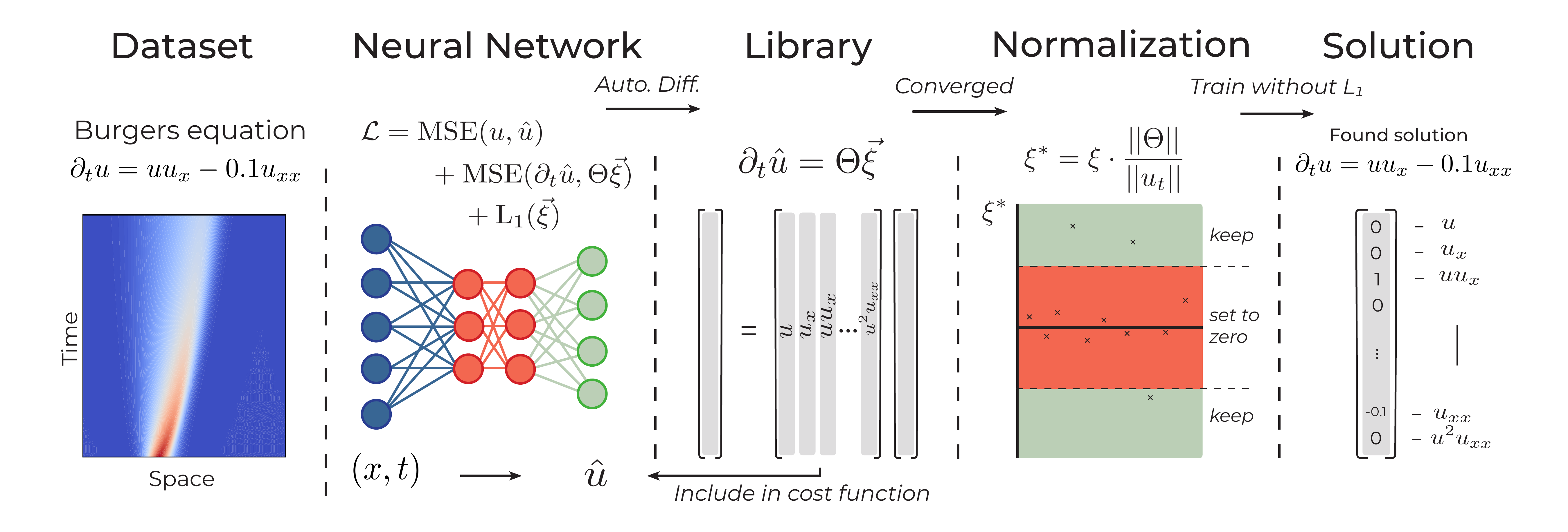
Figure 1: Schematic representation of the first DeepMoD iteration.

Results

We test the performance of this approach, which we call DeepMoD, on a set of case studies: the Burgers’ equation with and without shock, the 2D advection-diffusion equation and the Keller-Segel model for chemotaxis. These examples show the ability of DeepMoD to handle (1) non-linear equations, (2) solutions containing a shock wave, (3) coupled PDEs and finally (4) higher dimensional and experimental data.

Non-linear PDEs

The Burgers equation occurs in various areas of gas dynamics, fluid mechanics and applied mathematics and is evoked as a prime example to benchmark model discovery (Rudy et al. 2017; Long et al. 2017) and coefficient inference algorithms (Raissi, Perdikaris, and Karniadakis 2017a, 2017b), as it contains a non-linear term as well as second order spatial derivative, \[\begin{equation} \partial_t u = - u u_x + \nu u_{xx}. \label{eq:Burgers} \end{equation}\] Here \(\nu\) is the viscosity of the fluid and \(u\) its velocity field. We use the dataset produced by Rudy et al. (Rudy et al. 2017), where \(\nu=0.1\). The numerical simulations for the synthetic data were performed on a dense grid for numerical accuracy. DeepMoD requires significantly less datapoints than this grid and we hence construct a smaller dataset for DeepMoD by randomly sampling the results through space and time. From now on, we will refer to randomly sampling from this dense grid simply as sampling. Also note that this shows that our method does not require the data to be regularly spaced or stationary in time. For the data in Fig. 2 we add \(10\%\) white noise and sampled 2000 points for DeepMoD to be trained on.

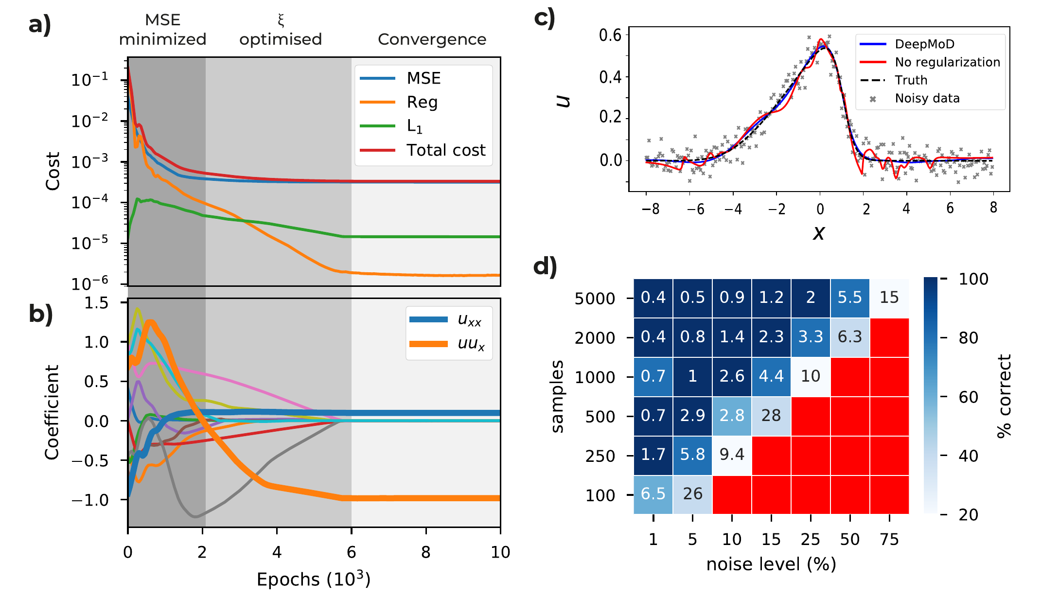
Figure 2: a) Cost functions and b) coefficient values as function of the number of epochs for the Burgers’ dataset consisting of 2000 points and 10% white noise. Initially, the neural network optimizes the MSE and only after the MSE is converged the coefficient vector is optimized by the network. c) Velocity field \(u\) for \(t = 5\) obtained after training with (no overfitting) and without (overfitting) the regression regularization \(\mathcal{L}_{Reg}\). d) The values in the grid indicate the accuracy of the algorithm tested on the Burgers’ equation, defined as the mean relative error over the coefficients, as function of the sample size of the data set and level of noise. The coloring represents the fraction of correct runs (Red indicates that in none of the five iterations the correct PDE is discovered).

We train the neural network using an Adam optimizer and plot the different contributions of the cost function as a function of the training epoch in Fig. 2a and we show the value of each component of \(\xi\) as a function of the training epoch in Fig. 2b. Note that for this example, after approximately 2000 epochs, the MSE is converged, while at the same time we observe the components of \(\xi\) only start to converge after this point. We can thus identify three ‘regimes’: in the initial regime (0 - 2000 epochs), the MSE is trained. Since the output of the neural network is far from the real solution, so is \(\Theta\), and the regression task cannot converge (See first 2000 epochs in Fig. 2b). After the MSE has converged, \(\hat{u}\) is sufficiently accurate to perform the regression task and \(\xi\) starts to converge. After this second regime (2000 - 6000 epochs), all components of the cost converged (>6000 epochs) and we can determine the solution. From this, we obtain a reconstructed solution (see Fig. 2b) and at the same time recover the underlying PDE, with coefficients as little as 1% error in the obtained coefficients. We show the impact of including the regression term in the cost function in Fig.2c, where the obtained solution of DeepMoD is compared with a neural network, solely trained on the MSE, to reconstruct the data. Including the regression term regularizes the network and prevents overfitting, despite the many terms in the library. We conclude that it is the inclusion of the regression in the neural network which makes DeepMoD robust to noisy data and prevents overfitting.

Next, we characterize the robustness of DeepMoD in Fig. 2d, where we run DeepMod for five times (differently sampled data set) for a range of sample sizes and noise levels. The color in Fig. 2d shows how many of the five runs return the correct equation and the value in the grid displays the mean error over all correct runs. Observe that at vanishing noise levels, we recover the Burgers equation with as little as 100 data-points, while for 5000 data points we recover the PDE with noise levels of up to 75%. Between the domain where we recover the correct equation for all five runs and the domain where we do not recover a single correct equation, we observe an intermediate domain where only a fraction of the runs return the correct equation, indicating the importance of sampling.

To benchmark DeepMoD, we can directly compare the performance of our algorithm with respect to two state-of-the-art methods, (i): PDE-Find by Rudy et al. (Rudy et al. 2017) and (ii) PDE-Stride by Maddu et al. (Maddu et al. 2019). Considering an identical Burgers’ data set with \(10^5\) data points, approach (i) recovers the correct equation for up to 1% Gaussian noise (Rudy et al. 2017) while method (ii) discovers the correct equation up to 5% noise (Maddu et al. 2019). Compared to the results in Fig. 2d we note that even for two order of magnitude fewer samples points, \(10^3\) w.r.t. \(10^5\), DeepMoD recovers the correct equation up to noise levels >50% Gaussian noise. DeepMoD allows up to two orders of magnitude higher noise-levels and smaller sample sizes with respect to state-of-the-art model discovery algorithms.

Shock wave solutions

If the viscosity is too low, the Burgers’ equation develops a discontinuity called a shock (See Fig. 3). Shocks are numerically hard to handle due to divergences in the numerical derivatives. Since DeepMoD uses automatic differentiation we circumvent this issue. We adapt the data from Raissi et al. (Raissi, Perdikaris, and Karniadakis 2017b) which has \(\nu=0.01/\pi\), sampling 2000 points and adding 10 \(\%\) white noise (See Fig. 3). We recover ground truth solution of the Burgers’ equation as well as the corresponding PDE, \[\begin{equation} \partial_t u = - 0.99 u u_x + 0.0035 u_{xx}, \end{equation}\] with a relative error of 5% on the coefficients. In Fig.3 we show the inferred solution for \(t=0.8\).

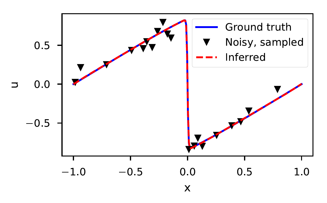
Figure 3: Ground truth, Noisy and Inferred data at \(t=0.8\) for the Burgers’ equation with a shock wave (10% noise and 2000 sample points).

Coupled differential equations

Next, we apply DeepMod to a set of coupled PDE’s in the form of the Keller-Segel (KS) equations, a classical model for chemotaxis (Painter 2018). Chemotactic attraction is one of the leading mechanisms that accounts for the morphogenesis and self-organization of biological systems. The KS model describes the evolution of the density of cells \(u\) and the secreted chemical \(w\), \[\begin{equation} \begin{split} \partial_t u = \nabla \cdot \left( D_u \nabla u - \chi u \nabla w \right) \\ \partial_t w = D_w \Delta w - k w + h u. \end{split} \end{equation}\] Here the first equation represents the drift-diffusion equation with a diffusion coefficient of the cells, \(D_u\) and a chemotactic sensitivity \(\chi\), which is a measure for the strength of their sensitivity to the gradient of the secreted chemical \(w\). The second equation represents the reaction diffusion equation of the secreted chemical \(w\), produced by the cells at a rate \(h\) and degraded with a rate \(k\). For a 1D system, we sample 10000 points of \(u\) and \(w\) for parameter values of \(D_u = 0.5\), \(D_v = 0.5\), \(\chi = 10.0\), \(k = 0.05\) and \(h = 0.1\) and add 5% white noise. We choose a library consisting of all spatial derivatives (including cross terms) as well as first order polynomial terms, totalling 36 terms. For these conditions we recover the correct set of PDEs, \[\begin{equation} \begin{split} \partial_t u = 0.50 u_{xx} - 9.99 u w_{xx} - 10.02 u_x w_x\\ \partial_t w = 0.48 w_{x x} - 0.049 w + 0.098 u, \end{split} \end{equation}\] as well as the reconstructed fields for \(u\) and \(w\) (See Fig. 4). Note that even the coupled term, \(u_x w_x\) , which becomes vanishingly small over most of the domain, is correctly identified by the algorithm, even in the presence of considerable noise levels.

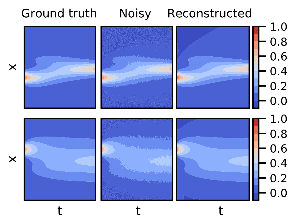
Figure 4: Ground truth, noisy and reconstructed solutions for the density of cells, \(u\) (top row) and the density of secreted chemicals \(w\) (bottom row) in the Keller Segel model for 5% white noise and 10000 samples.

Experimental data

To showcase the robustness of DeepMoD on high-dimensional and experimental input data, we consider a 2D advection diffusion process described by, \[\begin{equation} \partial_t u = -\nabla\cdot\left(-D\nabla u + \vec{v} \cdot u \right), \label{Eq:AdvectionDiffusion} \end{equation}\] where \(\vec{v}\) is the velocity vector describing the advection and \(D\) is the diffusion coefficient. In the SI of the paper we apply DeepMod on a simulated data-set of eq. , with as initial condition, a 2D Gaussian with \(D = 0.5\) and \(\vec{v} = (0.25,0.5)\). For as little as 5000 randomly sampled points we recover the correct form of the PDE as well as the vector \(\vec{v}\) for noise levels up to \(\approx\) 25%. In the absence of noise the correct equation is recovered with as little as 200 sample points through space and time. This number is surprisingly small considering this is an 2D equation.

Finally, we apply DeepMoD on a time-series of images from an electrophoresis experiment, tracking the advection-diffusion of a charged purple loading dye under the influence of a spatially uniform electric field. In Fig. 5a we show time-lapse images of the experimental setup where we measure the time-evolution of two initial localised purple dyes. Fig. 5b shows the resultant 2D density field for three separate time-frames (in arbitrary units), corresponding to the red square in Fig. 5a by substracting the reference image (no dye present). The dye displays a diffusive and advective motion with constant velocity \(v\), which is related to the strength of the applied electric field.

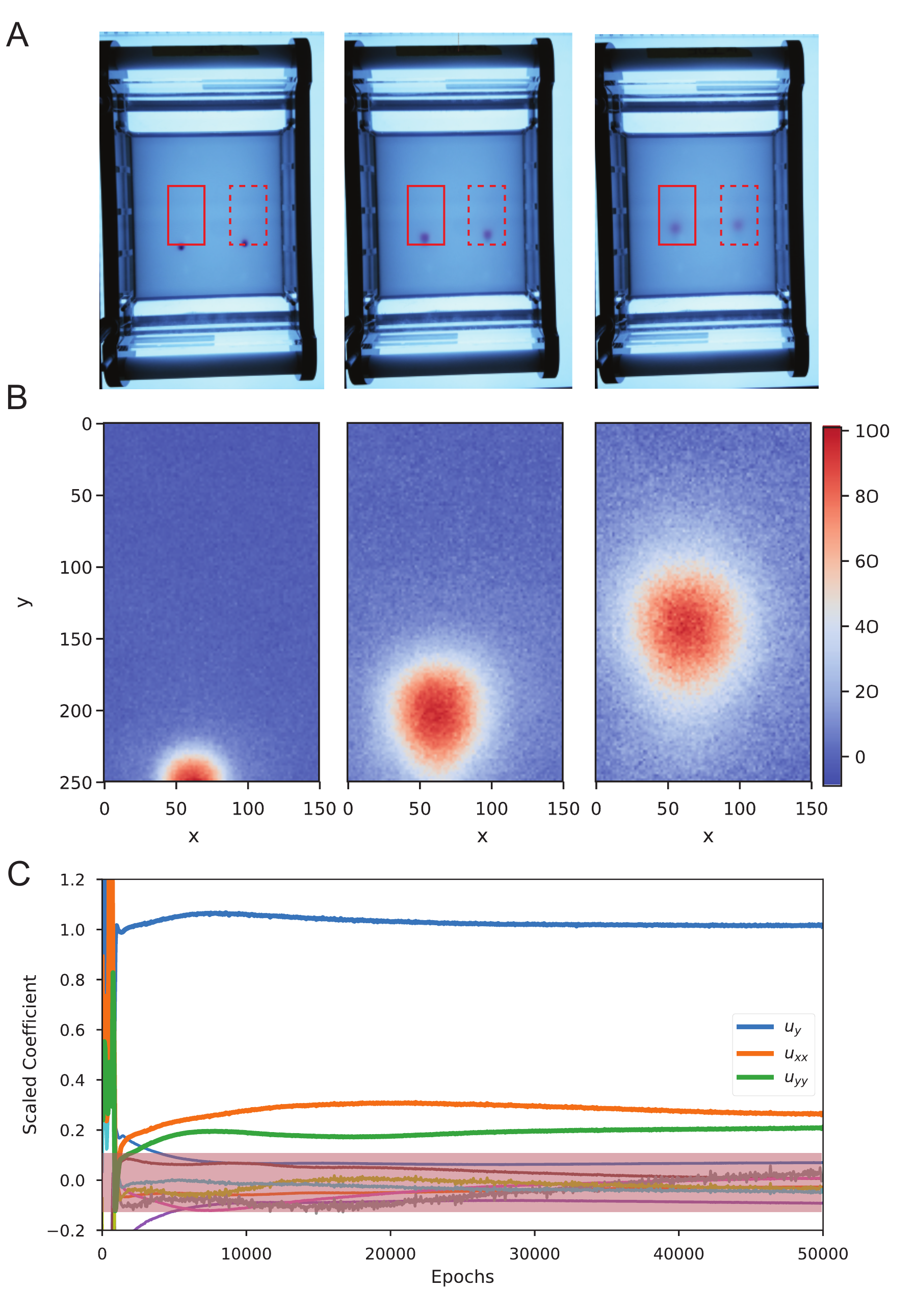
Figure 5: a) Time-serie images of the electrophoresis essay. The two red boxes indicate the analysed region. b) Region indicated in the solid red box of (a) showing the density of the dye at three different time-frames (in pixels). c) Scaled coefficients values of all the candidate for a single run. The pink region indicates the terms with scaled coefficient \(| \xi | < 0.1\).

We apply DeepMoD on 5000 sampled data-points sampled through space and time and consistently recover the advection term \(u_y\) as well as the two diffusive components (\(u_{xx}\) and \(u_{yy}\)). In Fig. c we show the scaled coefficients as function of the number of epochs. After thresholding the scaled coefficients (\(|\xi| < 0.1\)), we obtain for thre unscaled coefficients, the resultant advection diffusion equation, \[\begin{equation} 0.31 u_y + 0.011 u_{xx} + 0.009 u_{yy} = 0. \end{equation}\]

Analysing the second diffusing dye (dashed box in Fig. 5) result in nearly identical values for the drift velocity, \(v \approx 0.3\), and the diffusion coefficients, \(D \approx 0.01\) indicating the robustness of the obtained value of \(D\) and \(v\). In contrast to the artificial data presented in previous paragraphs, some higher-order non-linear terms, in particular \(u u_{yy}\) and \(u u_{xx}\) remain small, yet non-zero. This suggests that an automatic threshold strategy may not guarantee the desired sparse solution. Fixing a threshold of the scaled coefficients (\(|\xi| < 0.1\) in this particular case) or other thresholding strategies such as coefficient cluster detection would be better suited for this task.

Sparsely constrained neural networks for model discovery of PDEs

Gert-Jan Both, Gijs Vermarien, Remy Kusters - PDF

The original DeepMoD outperformed other model discovery approaches, but left several questions unanswered. Specifically, we wondered:

• How can the optimal strength of \(\ell_1\) penalty, \(\lambda\), be determined? Retraining the network would be prohibitively expensive, and while performance was not extremely sensitive to the choice of \(\lambda\), it is a hyperparameter which much be correctly chosen.
• Lasso has several undesirable properties and perhaps suboptimal performance. Can other model discovery algorithms such as SINDy be integrated in this framework?
• We never remove terms from the equation; rather, they approach or become zero due to the \(\ell_1\) penalty. Can performance be improved further removing the zero components and iteratively refining the estimate, similar to the iterative regression technique?

This paper was conceived and written mostly during the first confinement in Paris - plenty of time to think and wonder!

Next to answering these questions, this paper also represented a deepening of our understanding of the DeepMoD framework. We realized the coefficient vector \(\xi\) essentially performs two tasks: 1) selecting which terms are active, i.e. the ‘model discovery’ task and 2) constraining the neural network. The main innovation in this paper is the introduction of a mask \(g\) defining the support of \(\xi\), allowing us to separate these two tasks:

\[\begin{align} \mathcal{L}(\theta, \xi) = \sum_i \left\lVert u_i - \hat{u}_i \right\rVert^2_2 + \sum_i \left\lVert u_t - \Theta (g \cdot \xi) \right\rVert^2_2. \tag{3} \end{align}\]

This mask \(g\) is calculated non-differentiably, i.e. it effectively acts as an external ‘forcing variable.’ In ML applications, non-differentiability is typically considered a short-fall (see next section), but here it forms a bridge between neural-network based approaches and classical approaches. It is through the mask \(g\) that any sparse regression method can be utilized to perform variable selection on a neural-network based library. For example, lasso with cross validation can be used, but we also show an example with SINDy. We thus show that deep-learning based and classical methods can be synthesized, benefitting from both approaches. Together with this innovation we present a modular version of our framework, reprinted in figure 6.

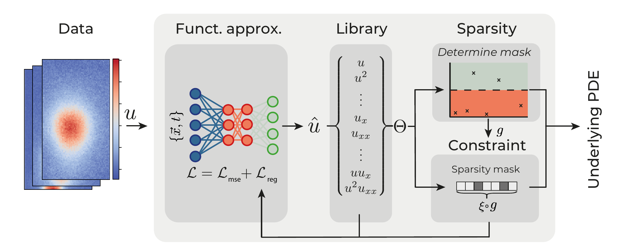
Figure 6: Schematic representation of the modular DeepMoD approach.

In this framework, (I) A function approximator constructs a surrogate model of the data, (II) from which a library of possible terms and the time derivative is constructed using automatic differentiation. (III) A sparsity estimator constructs the sparsity mask \(g\) to select the active terms in the library using some sparse regression algorithm and (IV) a constraint constrains the function approximator to solutions allowed by the active terms obtained from the sparsity estimator.

We released this paper together with a pytorch-based framework, DeePyMoD. Overall the paper and the software package made our approach significantly more flexible: each module can be easily changed, independent of another.

Results

Constraint

The sparse coefficient vector \(\xi\) in eq. (3) is typically found by optimising it concurrently with the neural network parameters \(\theta\). Considering a network with parameter configuration \(\theta^*\), the problem of finding \(\xi\) can be rewritten as \(\min_{\xi} \left|u_t(\theta^*) - \Theta (\theta^*)\xi\right|^2\). This can be analytically solved by least squares under mild assumptions; we calculate \(\xi\) by solving this problem every iteration, rather than optimizing it using gradient descent. In figure 7 we compare the two constraining strategies on a Burgers data-set, by training for 5000 epochs without updating the sparsity mask. Panel A) shows that the least-squares approach reaches a consistently lower loss. More strikingly, we show in panel B) that the mean absolute error in the coefficients is three orders of magnitude lower. We explain the difference as a consequence of the random initialisation of \(\xi\): the network is initially constrained by incorrect coefficients, prolonging convergence. The random initialisation also causes the larger spread in results compared to the least squares method. The least squares method does not suffer from sensitivity to the initialisation and consistently converges.

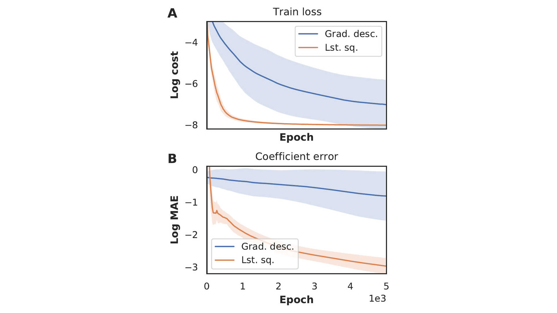
Figure 7: Loss and mean absolute error of the coefficients obtained with the gradient descent and the least squares constraint as a function of the number of epochs. Results have been averaged over twenty runs and shaded area denotes the standard deviation.

Sparsity estimator

Implementing the sparsity estimator separately from the neural network allows us to use any sparsity promoting algorithm. Here we show that a classical method for PDE model discovery, PDE-find (Rudy et al. 2017), can be used together with neural networks to perform model discovery in highly sparse and noisy data-sets. We compare it with the thresholded Lasso approach in figure 8 on a Burgers data-set with varying amounts of noise. The PDE-find estimator discovers the correct equation in the majority of cases, even with up to 60% - 80% noise, whereas the thresholded lasso mostly fails at 40%. We emphasise that the modular approach we propose here allows to combine classical and deep learning-based techniques. More advanced sparsity estimators such as SR3 (Champion et al. 2019) can easily be included in this framework.

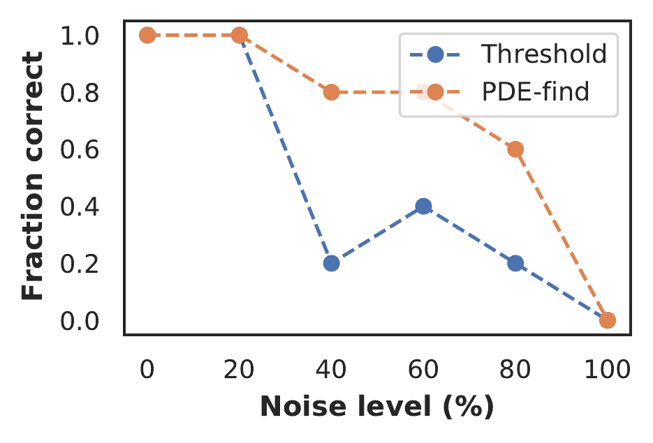
Figure 8: Fraction of correct discovered Burgers equations (averaged over 10 runs) as function of the noise level for the thresholded lasso and PDE-find sparsity estimator.

Function approximator

We show in figure 9 that a tanh-based NN fails to converge on a data-set of the Kuramoto-Shivashinksy (KS) equation (panel A and B). Consequently, the coefficient vectors are incorrect (Panel D). As our framework is agnostic to the underlying function approximator, we instead use a SIREN (Sitzmann et al. 2020), which is able to learn very sharp features in the underlying dynamics. In panel B we show that a SIREN is able to learn the complex dynamics of the KS equation and in panel C that it discovers the correct equation¹. This example shows that the choice of function approximator can be a decisive factor in the success of neural network based model discovery. Using our framework we can also explore using RNNs, Neural ODEs (Rackauckas et al. 2020) or Graph Neural Networks (Seo and Liu 2019).

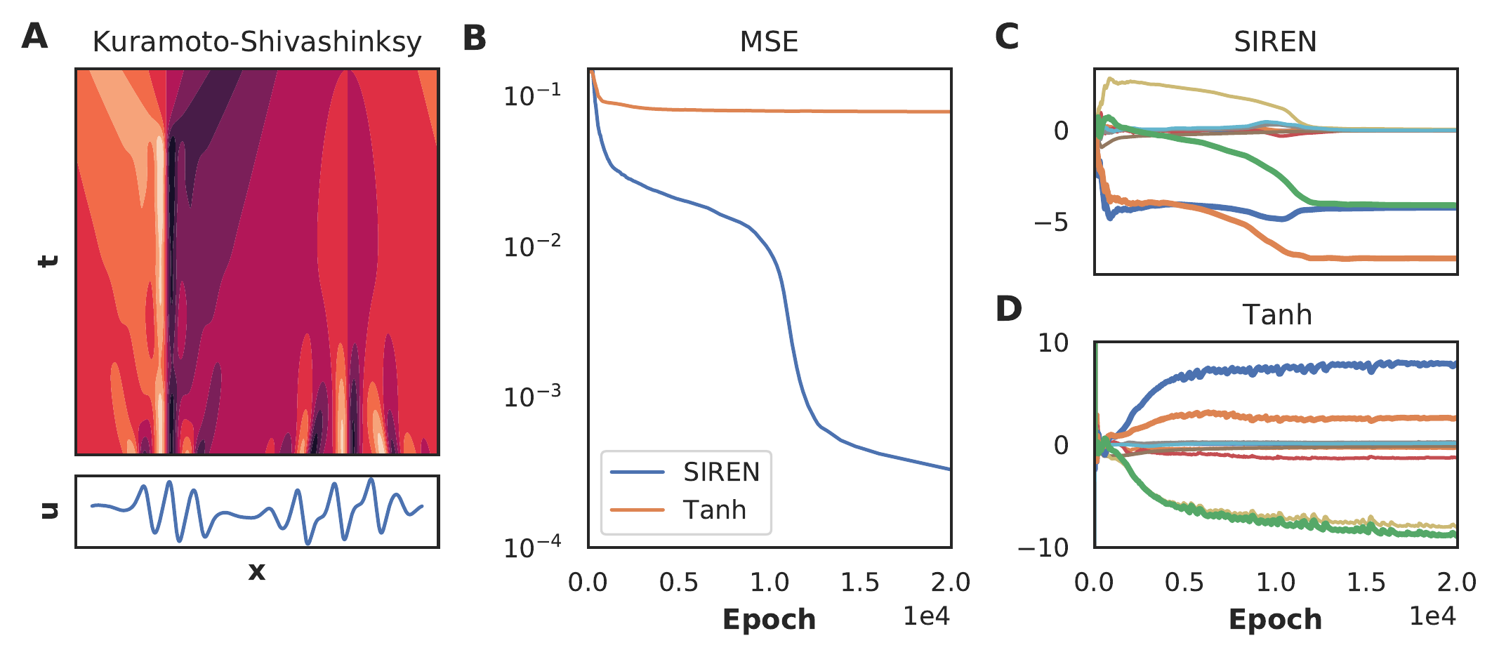
Figure 9: A Solution of the KS equation. Lower panel shows the cross section at the last time point: \(t=44\). B MSE as function of the number of epochs for both the tanh-based and SIREN NN. C Coefficients as function of number of epochs for the SIREN and D the tanh-based NN. The bold curves in panel C and D are the terms in the KS equation components; green: \(u u_x\):, blue: \(u_{xx}\) and orange: \(u_{xxxx}\). Only SIREN is able to discover the correct equation.

Fully differentiable model discovery

Gert-Jan Both, Remy Kusters - PDF

The modular approach in the second paper improved flexibility and performance, but left several things to be desired:

• It required the tuning of a fairly large set of hyperparameters: when to first update the mask, when to update it after, and which sparse regression approach to use (which itself introduces various hyperparameters).
• The non-differentiability of the mask allows to easily incorporate various sparse regression techniques, but also presents a weakness. If it is set incorrectly (for any reason), the training fails as the constraint is incompatible with the data. Additionally, due to this non-differentiability, model selection is effectively a side-effect of the training, and we hypothesize a fully differentiable method would increase performance and stability.

In this paper we create a fully-differentiable model discovery algorithm, which, considering eq. (3), requires making the mask \(g\) differentiable. Differentiable masking is challenging due to the binary nature of the problem, and instead we relax the application of the mask to a regularisation problem. Specifically, we propose to use Sparse Bayesian Learning (Tipping 2001) to select the active features and act as constraint.

This is my favourite paper. I think it’s an elegant approach solving many of the issues and questions of our previous papers, and as a bonus it also works in practice!

PINNs constrained by Sparse Bayesian Learning

Sparse Bayesian Learning (SBL) is a Bayesian approach to regression yielding sparse results. SBL defines a hierarchical model, starting with a Gaussian likelihood with noise precision \(\beta \equiv \sigma^{-2}\), and a zero-mean Gaussian with precision \(\alpha_j\) on each component \(\xi_j\) as prior, \[\begin{align} p(\partial_t \hat{u}; \ \Theta, \xi, \beta) = \prod_{i=1}^{N} \mathcal{N}(\partial_t \hat{u}_{i}; \ \Theta_i \xi, \beta^{-1}), \\ p(\xi ; \ A) =\prod_{j=1}^M \mathcal{N}(\xi_j ; \ 0, \alpha_j^{-1}), \end{align}\] with \(\partial_t \hat{u} \in \mathcal{R}^{N}\), \(\Theta \in \mathcal{R}^{N \times M}\), \(\xi \in \mathcal{R}^{M}\), and we have defined \(A \equiv \text{diag}(\alpha)\). The posterior distribution of \(\xi\) is a Gaussian with mean \(\mu\) and covariance \(\Sigma\), \[\begin{equation} \begin{split} \Sigma & = (\beta \Theta^T \Theta + A)^{-1}\\ \mu & = \beta \Sigma \Theta^T \partial_t\hat{u}. \end{split} \end{equation}\] Many of the terms in \(A\) will go to infinity when optimised, and correspondingly the prior for term \(j\) becomes a delta peak. We are thus certain that that specific term is inactive and can be pruned from the model. This makes SBL a very suitable choice for model discovery, as it gives a rigorous criterion for deciding whether a term is active or not. Additionally it defines hyper-priors over \(\alpha\) and \(\beta\), \[\begin{equation} \begin{split} p(\alpha) &= \prod_{j=1}^{M} \Gamma(\alpha_j ; \ a, b) \\ p(\beta) &= \Gamma(\beta ; \ c, d) \end{split} \end{equation}\] The inference of \(A\) and \(\beta\) cannot be performed exactly, and SBL uses type-II maximum likelihood to find the most likely values of \(\hat{A}\) and \(\hat{\beta}\) by minimising the negative log marginal likelihood²

\[\begin{equation} \mathcal{L}_{\text{SBL}}(A, \beta) = \frac{1}{2}\left[ \beta \left\lVert u_t - \Theta \mu \right\rVert^2 + \mu^T A \mu - \log\lvert \Sigma \rvert - \log \lvert A \rvert - N \log \beta \right]\\ - \sum_{j=1}^{M}(a \log\alpha_j - b \alpha_j) - c \log \beta + d \beta, \tag{4} \end{equation}\]

using an iterative method (see Tipping (2001)). The marginal likelihood also offers insight how the SBL provides differentiable masking. Considering only the first two terms of eq. (4), \[\begin{equation} \beta \left\lVert u_t - \Theta \mu \right\rVert^2 + \mu^T A \mu \end{equation}\] we note that the SBL essentially applies a coefficient-specific \(\ell_2\) penalty to the posterior mean \(\mu\). If \(A_j \to \infty\), the corresponding coefficient \(\mu_j \to 0\), pruning the variable from the model. Effectively, the SBL replaces the discrete mask \(m_j \in \{0, 1\}\) by a continuous regularisation \(A_j \in (0, \infty]\), and we thus refer to our approach as continuous relaxation.

Model

To integrate SBL as a constraint in PINNs, we place a Gaussian likelihood on the output of the neural network, \[\begin{equation} \hat{u}: p(u; \ \hat{u}, \tau) = \prod_{i=1}^{N}\mathcal{N}(u_i; \ \hat{u}_i,\ \tau^{-1}), \end{equation}\] and define a Gamma hyper prior on \(\tau\), \(p(\tau) = \Gamma(\tau ; \ e, f)\), yielding the loss function,

\[\begin{equation} \mathcal{L}_{\text{data}}(\theta, \tau) = \frac{1}{2}\left[ \tau \left\lVert u - \hat{u} \right\rVert^2 - N \log \tau\right] - e \log \tau + f \tau. \tag{5} \end{equation}\]

Assuming the likelihoods factorise, i.e. \(p(u, u_t ; \ \hat{u}, \ \Theta,\ \xi) = p(u ; \ \hat{u}) \cdot p(u_t ; \Theta, \ \xi)\), SBL can be integrated as a constraint in a PINN by simply adding the two losses given by eq. (4) and eq. (5), \[\begin{equation} \mathcal{L}_{\text{SBL-PINN}}(\theta, A, \tau, \beta) = \mathcal{L}_{\text{data}}(\theta, \tau) + \mathcal{L}_{\text{SBL}}(\theta, A, \beta) \end{equation}\] Our approach does not rely on any specific property of the SBL, and thus generalises to other Bayesian regression approaches.

Training

The loss function for the SBL-constrained PINN contains three variables which can be exactly minimised, and denote these as \(\hat{A}, \hat{\tau}\) and \(\hat{\beta}\). With these values, we introduce \(\tilde{\mathcal{L}}_{\text{SBL-PINN}}(\theta) \equiv \mathcal{L}_{\text{SBL-PINN}}(\theta, \hat{A}, \hat{\tau}, \hat{\beta})\) and note that we can further simplify this expression as the gradient of the loss with respect to these variables is zero. For example, \(\nabla_\theta \mathcal{L}(\hat{A})= \nabla_{A}\mathcal{L} \cdot \nabla_\theta A |_{A=\hat{A}} = 0\), as \(\nabla_A \mathcal{L} |_{A = \hat{A}} =0\). Thus, keeping only terms directly depending on the neural network parameters \(\theta\) yields,

\[\begin{equation} \begin{split} \tilde{\mathcal{L}}_{\text{SBL-PINN}}(\theta) & = \frac{\hat{\tau}}{2} \left\lVert u - \hat{u} \right\rVert^2 + \frac{\hat{\beta}}{2} \left\lVert u_t -\Theta \mu \right\rVert^2 + \mu^T \hat{A} \mu - \log\lvert \Sigma \rvert \\ & = \frac{N\hat{\tau}}{2}\underbrace{\left[\mathcal{L}_{\text{fit}}(\theta) + \frac{\hat{\beta}}{\hat{\tau}} \mathcal{L}_{\text{reg}}(\theta, \mu) \right]}_{=\mathcal{L}_{\text{PINN}}(\theta, \mu)} + \mu^T \hat{A} \mu -\log\lvert \Sigma \rvert \end{split} \tag{6} \end{equation}\]

where in the second line we have rewritten the loss function in terms of a classical PINN with relative regularisation strength \(\lambda = \hat{\beta} / \hat{\tau}\) and coefficients \(\xi = \mu\). Contrary to a PINN however, the regularisation strength is inferred from the data, and the coefficients \(\mu\) are inherently sparse.

An additional consequence of \(\nabla_\theta \mathcal{L}(\hat{A},\hat{\beta}, \hat{\tau})= 0\) is that our method does not require backpropagating through the solver. While such an operation could be efficiently performed using implicit differentiation (Bai, Kolter, and Koltun 2019), our method requires solving an iterative problem only in the forward pass. During the backwards pass the values obtained during the forward pass can be considered constant.

Considering eq. (6), we note the resemblance to multitask learning using uncertainty, introduced by Cipolla, Gal, and Kendall (2018). Given a set of objectives, the authors propose placing a Gaussian likelihood on each objective so that each task gets weighed by its uncertainty. The similarity implies that we are essentially reinterpreting PINNs as Bayesian or hierarchical multi-task models.

Physics Informed Normalizing Flows

Having redefined the PINN loss function in terms of likelihoods (i.e. eq. (6)) allows to introduce a PINN-type constraint to any architecture with a probabilistic loss function. In this section we introduce an approach with normalizing flows, called Physics Informed Normalizing Flows (PINFs). As most physical equations involve time, we first shortly discuss how to construct a time-dependent normalizing flow. We show in the experiments section how PINFs can be used to directly infer a density model from single particle observations.

Conditional Normalizing Flows

Normalizing flows construct arbitrary probability distributions by applying a series of \(K\) invertible transformations \(f\) to a known probability distribution \(\pi(z)\), \[\begin{equation} \begin{split} z & = f_K \circ \ldots \circ f_0(x) \equiv g_\theta(x)\\ \log p(x) & = \log \pi(z) + \sum_{k=1}^{K} \log \left \lvert \det \frac{\partial f_k(z)}{\partial dz} \right \rvert, \end{split} \end{equation}\] and are trained by minimising the negative log likelihood, \(\mathcal{L}_{\text{NF}} = -\sum_{i=1}^{N} \log p(x)\). Most physical processes yield time-dependent densities, meaning that the spatial axis is a proper probability distribution with \(\int p(x, t)dx=1\). Contrarily, this is not valid along the temporal axis, as \(\int p(x, t)dt = f(x)\). To construct PINFs, we first require a Conditional Normalizing Flow capable of modelling such time-dependent densities. Instead of following the method of , which modifies the Jacobian, we employ time-dependent hyper-network. This hyper-network \(h\) outputs the flow parameters \(\theta\), and is only dependent on time, i.e. \(\theta = h(t)\), thus defining a time-dependent normalizing flow as \(z = g_{h(t)}(x)\).

PINFs

Conditional normalizing flows yield a continuous spatio-temporal density, and the loss function of a PINF is defined as simply adding the SBL-loss to that of the normalizing flow, yielding \[\begin{equation} \tilde{\mathcal{L}}_{\text{PINF}}(\theta) = \mathcal{L}_{\text{NF}}(\theta) + \frac{N\hat{\beta}}{2} \mathcal{L}_{\text{reg}}(\theta, \mu) + \mu^T \hat{A} \mu -\log\lvert \Sigma \rvert. \end{equation}\]

Results

We now show several experiments illustrating our approach. We start this section by discussing choice of hyperprior, followed by a benchmark on several datasets and finally a proof-of-concept with physics-informed normalizing flows.

Choosing prior

The loss function for the SBL constrained approach contains several hyper-parameters, all defining the (hyper-) priors on respectively \(A\), \(\beta\) and \(\tau\). We set uninformed priors on \(A\) and \(\beta\), \(a=b=e=f=1e^{-6}\), but those on \(\beta\), the precision of the constraint, must be chosen more carefully. Figure illustrates the learning dynamics on a dataset of the Korteweg-de Vries equation when the \(\beta\) hyperprior is uninformed, i.e. \(c=d=1e^{-6}\). Observe that the model fails to learn the data, while almost immediately optimising the constraint. We explain this behaviour as a consequence of our assumption that the likelihoods factorise, which implies the two tasks of learning the data and applying the constraint are independent. Since the constraint contains much more terms than required, it can fit a model with high precision to any output the neural network produces. The two tasks then are not independent but conditional: a high precision on the constraint is warranted only if the data is reasonably approximated by the neural network. To escape the local minimum observed in figure , we couple the two tasks by making the hyper-prior on \(\beta\) dependent on the performance of the fitting task.

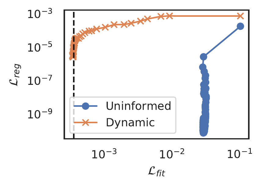
Figure 10: Regression loss as a function of fitting loss during training, comparing an uninformed prior with a dynamic prior.

Our starting point is the update equation for \(\beta\) (see Tipping (2001) for details), \[\begin{equation} \hat{\beta} = \frac{N - M + \sum_i \alpha_i \Sigma_{ii} +2c}{N \mathcal{L}_{\text{reg}} + 2d} \end{equation}\] We typically observe good convergence of normal PINNs with \(\lambda=1\), and following this implies \(\hat{\beta} \approx \hat{\tau}\), and similarly \(\mathcal{L}_{\text{reg}} \to 0\) as the model converges. Assuming \(N \gg M + \sum_i \alpha_i \Sigma_{ii}\), we have \[\begin{equation} \hat{\tau} \approx \frac{N + 2c}{2d}, \end{equation}\] which can be satisfied with \(c = N/2, \ d=n/\hat{\tau}\). Figure 10 shows that with this dynamic prior the SBL constrained PINN does not get trapped in a local minimum and learns the underlying data. We hope to exploit multitask learning techniques to optimize this choice in future work.

Experiments

We present three experiments to benchmark our approach. We first study the learning dynamics in-depth on a solution of the Korteweg- de Vries equation, followed by a robustness study of the Burgers equation, and finally show the ability to discover the chaotic Kuramoto-Shivashinsky equation from highly noisy data. Reproducibility details can be found in the appendix of the paper.

Korteweg-de Vries

The Korteweg-de Vries equation describes waves in shallow water and is given by \(u_t = u_{xxx} - u u_x\). Figure 11a shows the dataset: 2000 samples with 20% noise from a two-soliton solution. We compare our approach with I) Sparse Bayesian Learning with features calculated with numerical differentiation, II) a model discovery algorithm with PINNs, but non-differentiable variable selection called DeepMoD (Both and Kusters 2021) and III) PDE-find (Rudy et al. 2017), a popular model discovery method for PDEs based on SINDy (Brunton, Proctor, and Kutz 2016). The first two benchmarks also act as an ablation study: method I uses the same regression algorithm but does not use a neural network to interpolate, while method II uses a neural network to interpolate but does not implement differentiable variable selection.

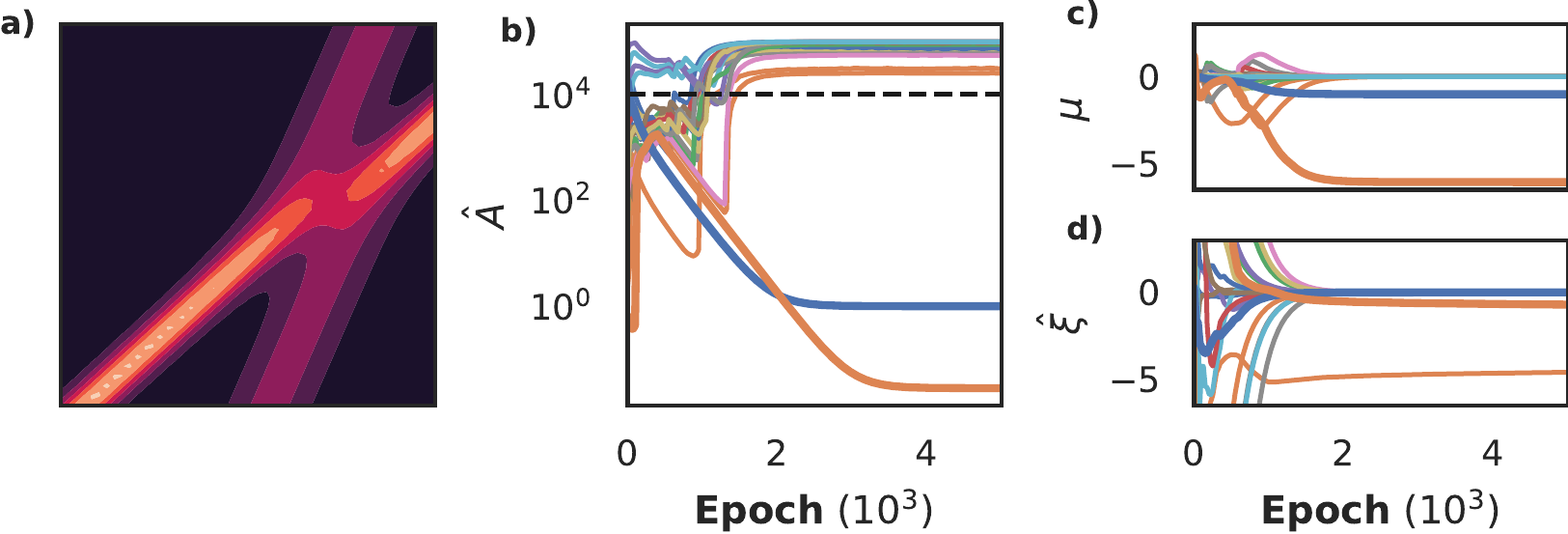
Figure 11: Comparison of a differentiable SBL-constrained model and an non-differentiable OLS-constrained model on a Korteweg-de Vries dataset (panel a) with a library consisting of 4th order derivatives and 3rd order polynomials, for a total of 20 candidate features. In panel b and c we respectively plot the inferred prior \(\hat{A}\) and the posterior coefficients \(\mu\). In panel d we show the non-differentiable DeePyMod approach. In panels b and c we see that the correct equation (bold blue line: \(u_{xx}\), bold orange line: \(uu_x\)) is discovered early on, while the non-differentiable model (panel d) selects the wrong terms.

In figure 11b and c we show that the differentiable approach recovers the correct equation after approximately 3000 epochs. Contrarily, DeepMoD recovers the wrong equation. Performing the inference 10 times with different seeds shows that the fully-differentiable approach manages to recover the Kortweg-de Vries equation nine times, while DeepMoD recovers the correct equation only twice - worse, it recovers the same wrong equation the other 8 times. Neither PDE-find nor SBL with numerical differentiation is able to discover the Korteweg-de Vries equation from this dataset, even at 0% noise due to the data sparsity.

Burgers

We now explore how robust the SBL-constrained PINN is with respect to noise on a dataset of the Burgers equation, \(u_t = \nu u_{xx} - u u_x\) (figure 12a). We add noise varying from 1% to 100% and compare the equation discovered by benchmark method II (DeepMoD, panel b) and our approach (panel c) - the bold orange and blue lines denote \(u_{xx}\) and \(uu_x\) respectively, and the black dashed line their true value. Observe that DeepMoD discovers small additional terms for >50% noise, which become significant when noise >80%. Contrarily, our fully differentiable approach discovers the same equation with nearly the same coefficients across the entire range of noise, with only very small additional terms (\(\mathcal{O}(10^{-4})\)). Neither PDE-find nor SBL with numerical differentiation is able to find the correct equation on this dataset at 10% noise or higher.

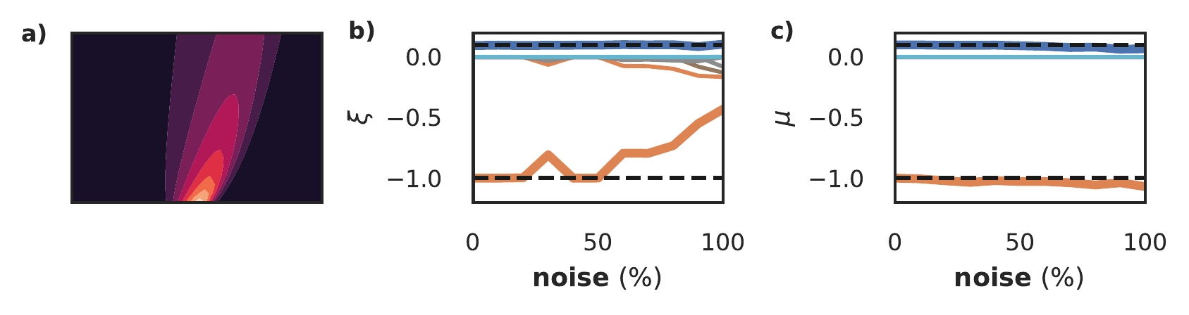
Figure 12: Exploration of robustness of SBL-constrained model for model discovery for the Burgers equation (panel a). We show the discovered equation over a range of noise for DeepMoD (panel b) and the approach presented in this paper (panel c). The bold orange and blue lines denotes \(u_xx\) and \(u u_x\), and black dashed line their true value.

Kuramoto-Shivashinsky

The Kuramoto-Shivashinksy equation describes flame propagation and is given by \(u_t = -uu_x - u_{xx} - u_{xxxx}\). The fourth order derivative makes it challenging to learn with numerical differentiation-based methods, while its periodic and chaotic nature makes it challenging to learn with neural network based methods (Both, Vermarien, and Kusters 2021). We show here that using the SBL-constrained approach we discover the KS-equation from only a small slice of the chaotic data (256 in space, 25 time steps), with 20% additive noise. We use a tanh-activated network with 5 layers of 60 neurons each, and the library consists of derivatives up to 5th order and polynomials up to fourth order for a total of thirty terms. Additionally, we precondition the network by training without the constraint for 10k epochs.

Training this dataset to convergence takes significantly longer than previous examples, as the network struggles with the data’s periodicity (panel b). After roughly 70k epochs, a clear separation between active and inactive terms is visible in panel c, but it takes another 30k epochs before all inactive terms are completely pruned from the model. Panels d and e show the corresponding posterior and the maximum likelihood estimate of the coefficients using the whole library. Remarkably, the MLE estimate recovers the correct coefficients for the active terms, while the inactive terms are all nearly zero. In other words, the accuracy of the approximation is so high, that least squares identifies the correct equation.

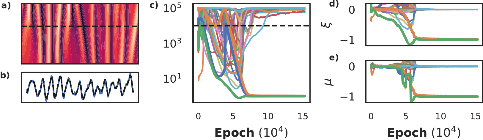
Figure 13: Recovering the Kuramoto-Shivashinsky equation. We show the chaotic data and a cross section in panels a and b. The periodicity makes this a challenging dataset to learn, requiring 200k iterations to fully converge before it can be recovered (panel c). Panels d and e show that the posterior and MLE of the coefficients yield nearly the same coefficients, indicating that the network was able construct an extremely accurate approximation of the data.

Model discovery with normalizing flows

Consider a set of particles whose movement is described by a micro-scale stochastic process. In the limit of many of such particles, such processes can often be described with a deterministic macro-scale density model, determining the evolution of the density of the particles over time. For example, a biased random walk can be mapped to an advection-diffusion equation. The macro-scale density models are typically more insightful than the corresponding microscopic model, but many (biological) experiments yield single-particle data, rather than densities. Discovering the underlying equation thus requires first reconstructing the density profile from the particles’ locations. Classical approaches such as binning or kernel density estimation are either non-differentiable, non-continuous or computationally expensive. Normalizing Flows (NFs) have emerged in recent years as a flexible and powerful method of constructing probability distribution, which is similar to density estimation up to a multiplicative factor. In this section we use physics informed normalizing flows to learn a PDE describing the evolution of the density directly from unlabelled single particle data.

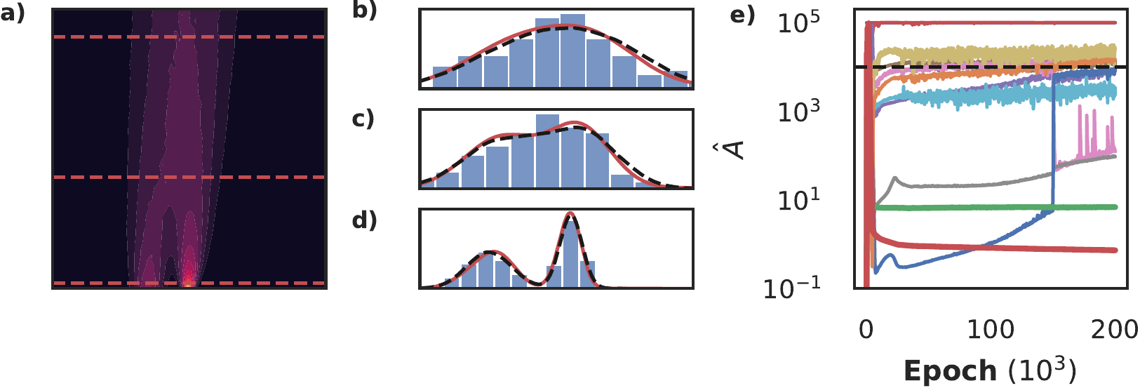
Figure 14: Using a tempo-spatial Normalizing Flow constrained by Sparse Bayesian Learning to discover the advection-diffusion equation directly from single particle data. Panel a shows the true density profile, and in panels b, c and d we show the density inferred by binning (blue bars), inferred by NF (red) and the ground truth (black, dashed) at \(t=0.1, 2.5, 4.5\). Note that although the estimate of the density is very good, we see in panel e that we recover two additional terms (bold blue line: \(u_x\), bold orange line \(u_{xx}\).

Since the conditional normalizing flow is used to construct the density, a precision denoting the noise level does not exist, and instead we set as prior for \(\beta\) \((a=N, b=N \cdot 10^{-5})\). We consider a flow consisting of ten planar transforms (Rezende and Mohamed 2015) and a hyper-network of two layers with thirty neurons each. The dataset consists of 200 walkers on a biased random walk for 50 steps, corresponding to an advection-diffusion model, with an initial condition consisting of two Gaussians, leading to the density profile shown in figure 14a. The two smallest terms in panel e correspond to the advection (bold green line) and diffusion (bold red line) term, but not all terms are pruned. Panels b, c and compare the inferred density (red line) to the true density (dashed black line) and the result obtained by binning. In all three panels the constrained NF is able to infer a fairly accurate density from only 200 walkers. We hypothesise that the extra terms are mainly due to the small deviations, and that properly tuning the prior parameters and using a more expressive transformation would prune the remaining terms completely. Nonetheless, this shows that NF flows can be integrated in this fully differentiable model discovery framework.

Temporal Normalizing Flows

Gert-Jan Both, Remy Kusters. PDF

In the biological sciences, single particle tracking (SPT) has become the method of choice to investigate many cellular processes. The obtained trajectories can be either analyzed as random walks, or from the perspective of walker densities. This density model is deterministic and typically more insightful than the stochastic random walk. However, in experiments the position of single particles, and from these positions a time-dependent density must be reconstructed. Classical methods such as binning or kernel density estimation are computationally expensive, non-differentiable,³ but above all unable to explicit model a time-dependent density. Rather, they construct snapshots of the density at given times. In this paper we introduce conditional normalizing flows (CNFs)⁴, a flexible and differentiable method which models the entire continuous spatio-temporal density.

This is another of my favourite papers. Although the execution leaves much to be desired, I believe the core idea is quite simple and elegant and can be of wide use.

We construct a Conditional Normalizing Flow by constraining the Jacobian of the transformation. Consider a two dimensional normalizing flow in spatial coordinate \(x\) and time \(t\):

\[\begin{align} p(x, t) = \pi(z, \tau) \left|\frac{dz}{dx}\frac{d\tau}{dt}-\frac{d\tau}{dx}\frac{dz}{dt} \right|, \quad [z,\tau] = f(x, t). \end{align}\]

\(z\) and \(\tau\) are thus some sort of latent coordinates. Since only the spatial axis represents a valid probability distribution, i.e. \(\int p(x, t) dx = 1\), but \(\int p(x, t) dt = f(x)\), only \(x\) can be validly transformed to \(z\). We enforce this by simply requiring \(t=\tau\), i.e. the latent time \(\tau\) is the real time \(t\). The transformation then reduces to

\[\begin{align} p(x, t) = \pi(z, t) \left|\frac{dz(x, t)}{dx} \right|, \quad z = f(x, t) \end{align}\]

i.e. the bijective transform depends on \(x\) and \(t\), but the coordinate \(t\) is not transformed.

Results

We now demonstrate tNFs on three datasets:

• A multi-scale toy problem to show tNFs can accommodate different length scales in a single distribution;
• A dataset of Brownian motion to show how tNFs enhance density estimation for sparse datasets;
• A dataset of chemotactic walkers to show that tNFs can correctly estimate a multi-modal, non-Gaussian density.

Multi-scale density estimation

A key problem in density estimation is inferring an accurate distribution when vastly different length scales are present within a single dataset. Classical approaches such as binning and KDE require a single characteristic length scale, prohibiting an accurate estimate of a multi-scale distribution. We now show that normalizing flows, and by extension tNFs, are capable of accurately inferring such a distribution.

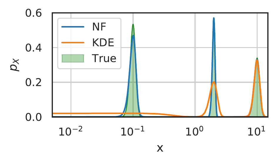
Figure 15: Comparison of density estimation with different scales. \(N=5000\) samples were taken from a density consisting of three Gaussians with widths \(0.01\), \(0.1\), and \(1\), at respective locations \(0.1, 2\) and \(10\), and weights \(0.013, 0.13\) and \(0.85\). The KDE used a Gaussian kernel with the kernel width set by Scott’s rule.

We build an artificial distribution consisting of three normal distributions with standard deviations \(\sigma\) of \(0.01, 0.1\) and \(1.0\) (thus spanning three orders of magnitude) and respective weights \(0.013, 0.13\) and \(0.85\). Figure 15 shows the inferred distribution from 5000 samples for the NF and the KDE with Scott’s rule determining the lengthscale. Observe that, as expected, the KDE is unable to accommodate the different scales and that due the different weighting of each peak, the widest is dominating the lengthscale estimation. Contrarily, the NF provide an accurate density estimate for all lengthscales present in the problem, independent of their weights. We stress that tNF do not require any prior information of the different lengthscales present in the data-set.

Brownian motion

Brownian motion is the most basic and ubiquitous random walk and thus an ideal test case to assess the performance of tNFs, comparing them to time independent NFs and classical binning. We generate a single trajectory for a Brownian random walker by the recursive relation, \(\vec{x}_{n+1} = \mathcal{N}(\vec{x}_n, \sqrt{2D\Delta t})\). Here \(n\) is the step number with \(x_0\) the initial position, \(D\) the diffusive coefficient and \(\Delta t\) the time step. In the limit of an infinite number of walkers, the walker density \(c\) is described by the diffusion equation, \(\partial_t c = D\nabla^2 c\).

Our dataset consists of \(M=500\) walkers with \(D=2.0\), with snapshots being taken every \(\Delta t = 0.1\) for \(N=100\) frames. The initial positions were sampled from a Gaussian centered at \(x=1.5\) with width \(\sigma=0.5\); in this case, the diffusion equation can be solved exactly and the solution behaves as a spreading Gaussian in time. We show the estimated density at \(t = 0.75\) and \(t = 4.25\) in figure (a) and (b) for the tNF, the time independent NF and binning. The tNF provides a significantly better density estimate than the time independent NF, illustrated by the difference in \(\ell_2\) error; \(2.6\cdot10^{-5}\) for the tNF and \(7.4\cdot10^{-5}\) for the NF, averaged over frame 15 and 85.

Normalizing flows are based on neural networks and hence prone to overfitting. We analyze the effect of overfitting in Appendix I of the paper and show that NFs overfit more strongly than tNFs and perform worse in terms of the \(\ell_2\) error. We mainly attribute this improvement to the temporal correlations in the dataset, which suppresses the natural frame-to-frame variations in the density estimate. Nonetheless, tNFs are not immune to overfitting and we speculate performance could be enhanced by applying techniques such as early stopping.

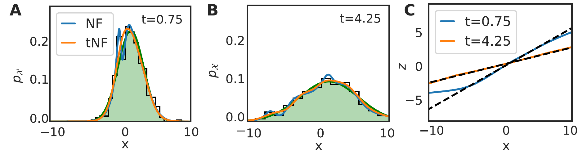
Figure 16: Results of inferring a Brownian walker density from \(M=500\) walkers with \(D=2\) and where a snapshot was taken every \(\Delta t=0.1\) for \(N=100\) frames. The initial position was sampled from a Gaussian placed at \(x=1.5\) with width \(\sigma=0.5\). Panel a and b compare the inferred density by binning, time independent normalizing flow (NF) and time dependent normalizing flow (tNF) at two different times. Panel c compares the learned mapping with the true mapping.

For the diffusion equation the true mapping can be trivially derived. We compare it to the learned mapping in figure 16c. It shows perfect agreement at \(t=4.25\), but deviates from the true curve for \(x<-5\) at \(t=0.75\). As can be seen in figure 16a, no samples were present in this domain, explaining the deviance. Nonetheless, it implies that the network does not generalize well outside the sampling domain. We speculate that techniques such as batch normalization or a different architecture for the network (a recurrent network, for example) might further improve performance.

Chemotaxis

The Brownian motion presented in the previous section was a linear problem with a uni-modal, Gaussian solution. We now apply tNFs to so-called chemotactic walkers, a non-linear problem with a multi-modal solution. Bacteria and other micro-organisms sense gradients of chemicals throughout their environment and use this to guide their motion towards a food source. This effect is known as chemotaxis and is typically modelled by a random walker with a superimposed drift; \(\vec{x}_{n+1} = \mathcal{N}(\vec{x}_n + \chi \nabla p(\vec{x}_n)dt, \sqrt{2Ddt})\), where \(p\) is the chemical density and \(\chi\) is the , which controls the interaction between the chemical and the bacteria. In the infinite walker limit, the walker and chemical density are given by the Keller-Segel model: \(\partial_t c = \nabla \cdot (D_c \nabla c - \chi c\nabla p)\) and \(\partial_t p = D_p \nabla^2 p - Kp\). Here \(D_c\) and \(D_p\) are the diffusion coefficients of the bacteria and the chemical respectively and a decay set by \(K\) has been added to the chemical density.

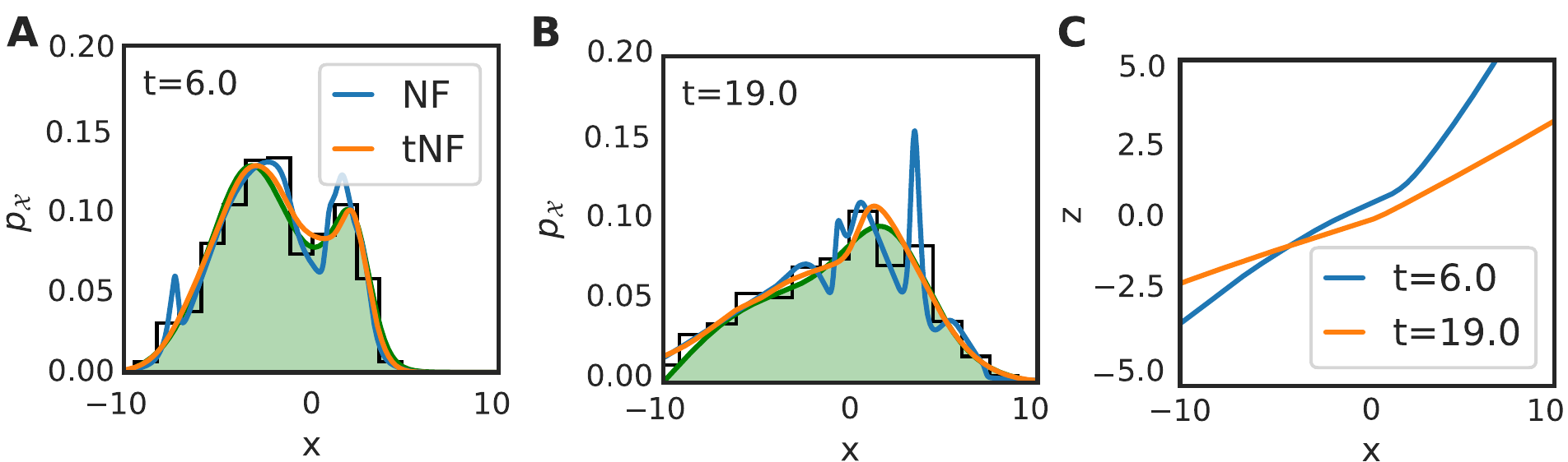
Figure 17: Results of inferring a chemotactic walker density from \(M=500\) walkers with \(D=0.5\) and chemotactic sensitivity \(\chi = 10\), where a snapshot was taken every \(\Delta t=0.1\) for \(N=100\) frames. The initial position was sampled from a Gaussian placed at \(x=-2.5\) with width \(\sqrt{0.5}\), while the food source is a Gaussian located at \(x=2.5\) with width \(\sqrt{0.5}\), diffusing with \(D=0.25\) and decaying at a rate of 0.05. Panel a and b compare the inferred density by binning, time independent normalizing flow (NF) and time dependent normalizing flow (tNF) at two different times. Panel c compares the learned mapping with the true mapping.

Our dataset consisted of \(M=500\) walkers with \(D=0.5\) and we sampled the initial position from a Gaussian centred at \(x=-2.5\). The food source was modelled by a Gaussian with diffusion coefficient \(D=0.25\), centred at \(x=2.5\); the walkers will thus drift towards food source over time. Figure 17 shows a comparison of the time independent NF, tNF and the binning method. In figure 17(a) and (b) we find that the tNF leads to a significantly more accurate density estimation, illustrated by the difference in \(\ell_2\) error (\(1.45\cdot10^{-4}\) for the NF versus \(1.8\cdot10^{-5}\) for the tNF, averaged over \(t=6.0\) and \(19.0\)). The tNF captures the multi-modal distribution at \(t=6.0\) excellently, without overfitting, contrarily to the time independent NF. The mapping, as shown in figure 17c, is non-linear, in contrast to the mapping obtained for the Brownian motion.

Model discovery in the sparse sampling regime

Gert-Jan Both, Georges Tod, Remy Kusters. PDF

DeepMoD can handle much sparser data than other classical interpolation techniques. In this paper we compare our method in-depth to spline interpolation, how it fails as data becomes sparser and link it to the data’s characteristic lengthscale.

This paper started with a curious observation: between our first and second paper we noticed a curious regression in performance. We eventually traced it back to a change in sampling strategy: when the data was randomly sampled instead of on a grid, DeepMoD was able to recover the underlying equation with much less data.

Results

Synthetic data - Burgers equation

We consider a synthetic data set of the Burgers equation \(u_t = \nu u_{xx} - u u_x\), with a delta peak initial condition \(u(x, t=0) = A \delta(x)\) and domain \(t \in [0.1, 1.1], x \in [-3, 4]\). This problem can be solved analytically to yield a solution dependent on a dimensionless coordinate \(z = x / \sqrt{4 \nu t}\). We recognize the denominator as a time-dependent length scale: a Burgers data set sampled with spacing \(\Delta x\) thus has a time-dependent dimensionless spacing \(\Delta z(t)\). We are interested in the smallest characteristic length scale, which for this data set is \(l_c = \sqrt{4 \nu t_0}\), where \(t_0=0.1\) is the initial time of the data set. We set \(A=1\) and \(\nu=0.25\), giving \(l_c = \sqrt{0.1} \approx 0.3\).

Splines do not scale effectively beyond a single dimension, making it hard to fairly compare across both the spatial and temporal dimensions. We thus study the effect of spacing only along the spatial axis and minimize the effect of discretization along the temporal axis by densely sampling 100 frames, i.e. \(\Delta t = 0.01\). Along the spatial axis we vary the number of samples between 4 and 40, equivalent to \(0.5 < \frac{\Delta x}{l_c} < 5\). We study the relative error \(\epsilon\) as the sum of the relative errors for all the derivatives, normalized over every frame,

\[\begin{equation} \epsilon = \sum_{i=1}^{3} \left\langle\frac{\left\lVert\partial_{x}^{i} u_j - \partial_{x}^i \hat{u}_j\right\rVert_2}{\left\lVert \partial_{x}^{i} u_j \right\rVert_2}\right\rangle_j \label{eq:error} \end{equation}\]

where \(i\) sums the derivatives and \(j\) runs over the frames. The derivatives are normalised every frame by the \(l_2\) norm of the ground truth to ensure \(\epsilon\) is independent of the magnitude of \(u\). \(\epsilon\) does not take into account the nature of noise (e.g. if it is correlated and non-gaussian), nor if the correct equation is discovered. However, taken together with a success metric (i.e if the right equation was discovered), it does serve as a useful proxy to the quality of the interpolation.

Figure b) shows \(\epsilon\) as a function of the relative spacing \(\Delta x / l_c\) and whether the correct equation was discovered. The error when using splines (yellow) increases with \(\Delta x\) and, as expected, we are unable to discover the correct equation for \(\Delta x > 0.8 l_c\) (dots indicate the correct equation is discovered and triangles indicates it failed to do so). Considering the NN-based DeepMoD method, sampled on a grid (green), we observe that it is able to accurately interpolate and discover the correct equation up to \(\Delta x \approx 1.2 l_c\). The reason for this is that NN-based interpolation constructs a surrogate of the data, informed by both the spatial and the temporal dynamics of the data set, while classical interpolation is intrinsically limited to a single time frame.

In figure 18c) we consider the same graph with 20% white noise on the data. Despite smoothing, the spline is unable to construct an accurate library and fails to discover the correct equation in every case. DeepMoD stands in stark contrast, discovering the correct equation with comparable relative error as in the 0% noise case.

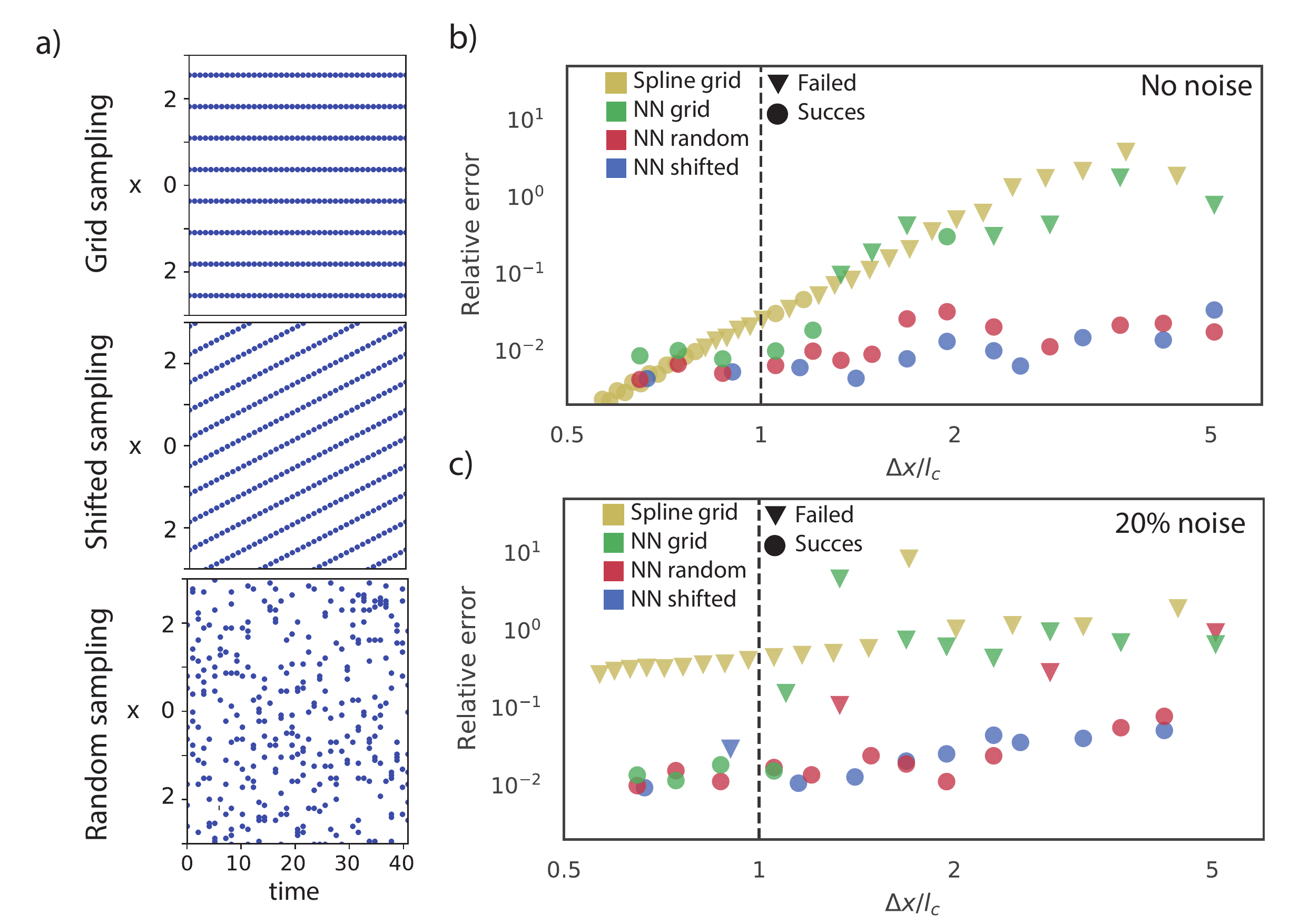
Figure 18: a) The three sampling strategies considered. b) and c) Error in the function library as function of the distance between the sensors \(\Delta x\), normalized with \(l_c = \sqrt{4 \nu t_0}\), for b) noise-less data and c) 20% of additive noise. The yellow symbols correspond to a spline interpolation and the green, blue and red correspond to the NN-based model discovery with various sampling strategies. The circles indicate that model discovery was successful while the triangles indicate that the incorrect model was discovered. The horizontal dashed line indicates the smallest characteristic length-scale in the problem: \(\Delta x / l_c = 1\).

Off-grid sampling

Whereas higher-order splines are constrained to interpolating along a single dimension, DeepMoD uses a neural network to interpolate along both the spatial and temporal axis. This releases us from the constraint of on-grid sampling, and we exploit this by constructing an alternative sampling method. We observe that for a given number of samples \(n\), DeepMoD is able to interpolate much more accurately if these samples are randomly drawn from the sampling domain. We show in figure 18b and c (Red) that the relative error \(\epsilon\) in the sparse regime, can be as much as two orders of magnitude lower compared to the grid-sampled results at the same number of samples. We hypothesize that this is due to the spatio-temporal interpolation of the network. By interpolating along both axes, each sample effectively covers its surrounding area, and by randomly sampling we cover more of the spatial sampling domain. Contrarily, sampling on a grid leaves large areas uncovered; we are effectively sampling at a much lower resolution than when using random sampling.

To test whether or not this improvement is intrinsically linked to the randomness of sampling, we also construct an alternative sampling method called shifted-grid sampling. Given a sampling grid with sensor distance \(\Delta x\), shifted-grid sampling translates this grid a distance \(\Delta a\) every frame, leading to an effective sample distance of \(\Delta a \ll \Delta x\). This strategy, similarly as random sampling varies the sensor position over time, but does so in a deterministic and grid-based way. We show this sampling strategy in figure 18a, while panels b and c confirm our hypothesis; shifted grid sampling (Blue) performs similarly to random sampling. Shifted-grid sampling relies on a densely sampled temporal axis ‘compensating’ for the sparsely sampled spatial axes. This makes off-grid sampling beneficial when either the time or space axis, but not both, can be sampled with a high resolution. In the experimental section we show that if both axes are sparsely sampled, we do not see a strong improvement over grid sampling.

Experimental data - 2D Advection-Diffusion

In an electrophoresis experiment, a charged dye is pipetted in a gel over which a spatially uniform electric field is applied (see Figure 19a)). The dye passively diffuses in the gel and is advected by the applied electric field, giving rise to an advection-diffusion equation with advection in one direction: \(u_t = D (u_{xx} + u_{yy}) + v u_y\). Both et al. (2019) showed that DeepMoD could discover the correct underlying equation from the full data-set (size 120 x 150 pixels and 25 frames). Here, we study how much we can sub-sample this data and still discover the advection-diffusion equation.

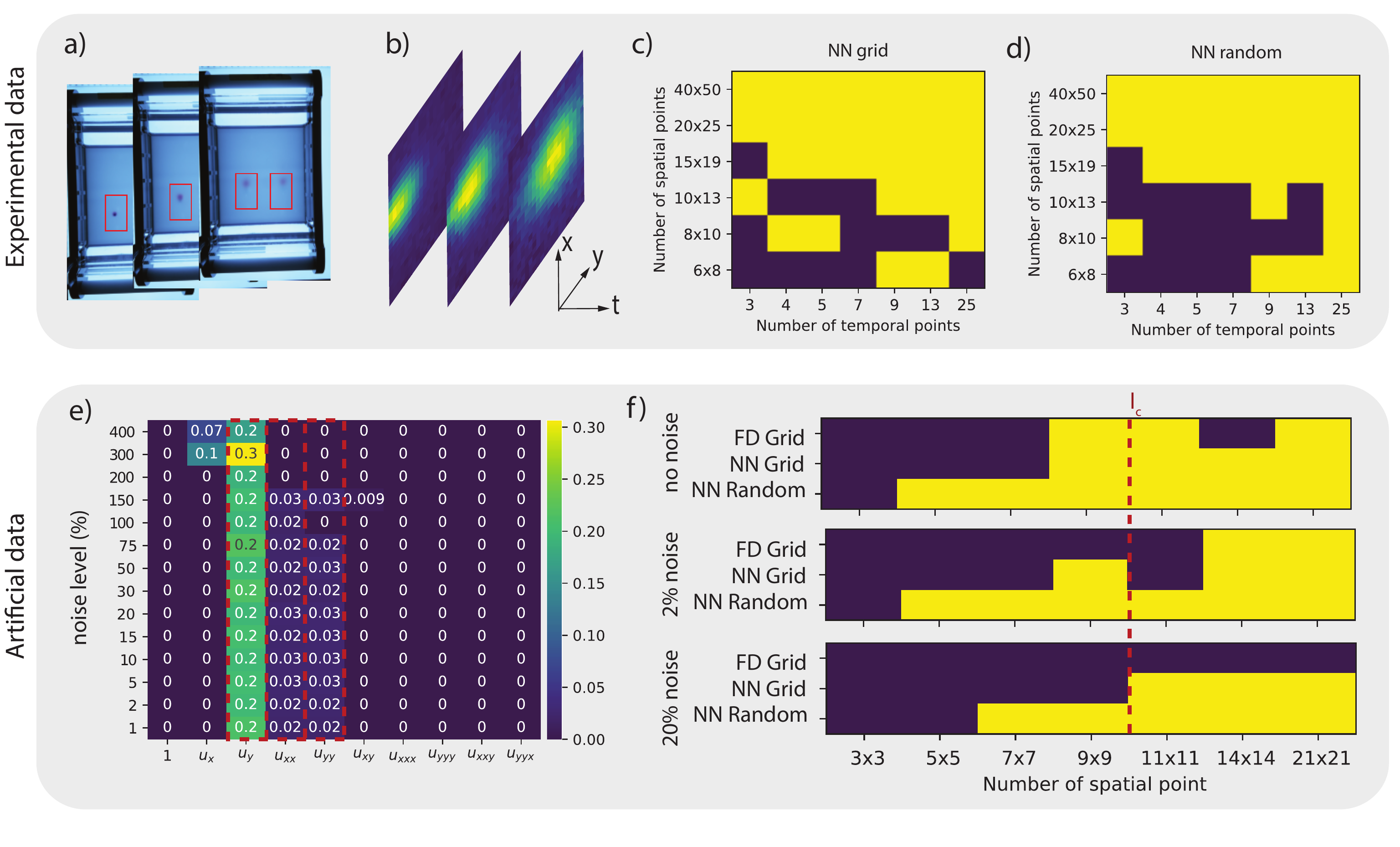
Figure 19: a) Experimental setup of the gel electrophoresis. b) Three time frames of the density with a spatial resolution of 20x25. c) and d) Success diagram for the experimental data indicating correct model discovery (Yellow indicates the correct AD equation \(u_t = D (u_{xx} + u_{yy}) + v u_y\) is discovered) as function of the spatial and temporal resolution for c) grid sampling and d) random sampling. e) Obtained mask and coefficients (\(D = 0.025\) and and \(v = (0, 0.2)\)) for the artificial data-set as function of the noise level (11x11 spatial resolution). Hereby, yellow indicates the terms selected by the algorithm and the red dashed box the terms that are expected in the PDE. f) Success diagrams for various levels of additive noise, comparing the result of DeepMoD with a grid and random sampling strategy and the classical LassoCV algorithm on a Finite Difference (FD)-based library (after SVD filtering of the different frames).

In figure 19 c) and d) we perform grid based as well as a random sub-sampling of the data. The neural network-based method discovers the advection-diffusion equation on as few as 6 x 8 spatial sampling points with 13 time-points, or with 20 x 25 pixels on only 3 time-points. The minimum number of required samples is similar for grid and random sampling, confirming that when both axes are poorly sampled, there is no benefit to sample randomly.

The smallest characteristic length scale in the problem is the width of the dye at \(t=t_0\), which we estimate as \(l_c \approx 10\) pixels. For the data presented in figure c) and 19d), at a resolution below \(10 \times 13\) sensors classical approaches would inherently fail, even if no noise was present in the data set. This is indeed what we observe: using a finite difference-based library we were unable to recover the advection-diffusion equation, even after denoising with SVD. However, we do observe that below this value we occasionally discover the correct PDE, despite the experimental noise present in the data. The use of a neural network and random sampling lead to non-deterministic behaviour: the neural network training dynamics depend on its initialization and two randomly sampled datasets of similar size might not lead to similar results. In practice this leads to a ‘soft’ decision boundary, where a fraction of a set of runs with different initialization and datasets fail.

Noiseless synthetic data set

To further confirm our results from the previous section, we simulate the experiment by solving the 2D advection-diffusion with a Gaussian initial condition and experimentally determined parameters (\(D = 0.025\) and and \(v = (0, 0.2)\). Figure 19e) shows the selected terms and their magnitude as functions of the applied noise levels for a highly subsampled data-set (grid sampling, spatial resolution of 11x11 and temporal resolution 14). The correct AD equation is recovered up to noise levels of 100\(\%\) (See figure 19e), confirming the noise robustness of the NN-based model discovery. In panel f) we compare the deep-learning based model discovery using grid and random sampling with classical methods for various noise levels and sensor spacing with a fixed temporal resolution of 81 frames (Data for the FD was pre-processed with a SVD filter, see SI for further details). We confirm that, similarly to the Burgers example of the previous section, the correct underlying PDE is discovered even below the smallest characteristic length-scale in the problem (indicated by a red dashed line in figure 19f).

This figure confirms our three main conclusions: 1) In the noiseless limit, classical approaches are only slightly less performing than NN-based model discovery for grid sampling. 2) Increasing the noise level dramatically impacts classical model discovery while barely impacting NN-based model discovery and 3) random sampling over space considerably improves performance, allowing model discovery with roughly 4-8 times fewer sample points for this particular data-set (depending on the noise level).

Experimental data - Cable equation

Applying a constant voltage to a RC-circuit with longitudinal resistance (see figure 20 a) result in time-dependent voltage increase throughout the circuit due to the charging of the capacitors. This rise is modeled by the cable equation, which is essentially a reaction-diffusion equation $ u_t = u_{xx}/ (R_l C) + u/(R_m C)$ with \(C\) the capacitance, \(R_l\) the longitudinal resistance and \(R_m\) the parallel resistance of the circuit. The discrete nature of the experiment automatically gives \(\Delta x = O(l_c)\). We consider an extreme case where we only have seven sensors throughout the circuit (i.e. spatial axis), but take 2500 samples along the time axis. Figure 20b shows the measured voltage at these seven elements. Initially, all the capacitors are uncharged and we observe a sharp voltage increase at the first element. As the capacitors charge, this further propagates through the circuit, charging the capacitors and resulting in the curves shown in the figure. We apply both a classical approach with the library generated with splines and DeepMoD to a varying amount of elements. Figure 20 c and d show that the DeepMoD discovers the cable equation with as few as seven elements, whereas classical methods are unable to find the cable equation at any number of elements.

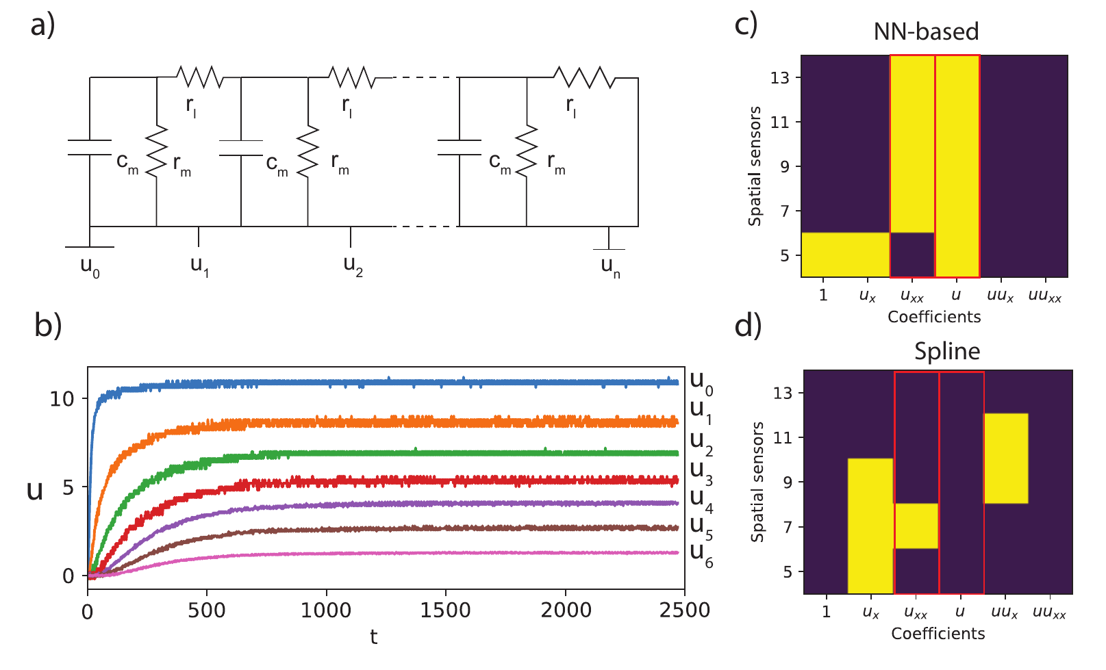
Figure 20: a) Schematic overview of the electronic setup to generate the cable equation. b) The voltage drop \(u\) as function of time for various positions along the circuit for a circuit with 7 elements. The mask obtained for c) NN-based and d) cross validated Lasso with spline based library model discovery (Yellow indicates the term was recovered by the algorithm). The red boxes indicate the two expected terms in the equation.

---

1. In bold; \(u u_x\): green, \(u_{xx}\): blue and \(u_{xxxx}\): orange↩︎

2. Neglecting the hyper-prior, this loss function can also written more compactly as \[\begin{equation} \mathcal{L}_{\text{SBL}}(A, \beta) = \log \left \lvert C \right \rvert + \partial_t u^T C^{-1}\partial_t u, \quad C = \beta^{-1} I + \Theta A^{-1} \Theta^T, \end{equation}\] but the format we use provides more insight how SBL provides differentiable masking.↩︎

3. meaning that the inferred density is a given and cannot be changed.↩︎

4. When we wrote this paper, we only considered dependence on time - hence the name temporal normalizing flow. Calling them CNFs generalizes our approach and brings it in line with literature.↩︎