Model discovery of partial differential equations

Model discovery aims at autonomously discovering equations underlying a dataset. It is often approached as a sparse regression problem, selecting terms and constructing the unknown equation from a set of candidate feautures. In the case of partial differential equations, these features consist of higher-order derivatives, which are calculated using numerical differentiation. This makes it challenging to accurately calculate the candidate feature in experimental data, which is noisy and sparse. In this thesis we develop a neural network-based model discovery method, with a focus on discovering partial differential equations from noisy and sparse data. The foundation of our approach is a neural network which interpolates and denoises the data, and constrain the network to a given equation - a model known as physics informed neural networks. Simultaneously, we employ sparse regression to learn this constraining equation as the neural network is trained, yielding the underlying model. In the first part of this thesis we show that such an approach significantly improves the robustness of model discovery compared to unconstrained neural networks or other model discovery approaches. Improving on this, in the second part we present a modular framework, showing how these constrained networks can utilize any sparse regression algorithm. In the third part, we build upon the first two parts to achieve a fully differentiable model discovery algorithm by constraining a neural network with Sparse Bayesian Learning. Additionally, we introduce Conditional Normalizing Flows and show how they can be used to infer time-dependent probability distributions. Taken together, our work shows the importance of accurately modelling data for model discovery, and strongly establishes the argument for physics-constrained, neural network-based surrogates for model discovery of PDEs on experimental data.

Figure 1: One-dimensional solution of the Kuramoto-Shivashinsky equation.

How much can a picture tell us? The image above shows an initial disturbance slowly breaking up into many small waves, which themselves merge and split as time progresses. Such complex behaviour is certainly beautiful to behold, but as scientists we wish take it a step further. Can we understand the underlying system and capture it in a (quantitative) model? This seems a daunting task considering figure 1, yet this process is at the heart of science. The classical approach to construct such models is known as First-Principle modelling. It starts, as the name implies, from basic principles and relies on simple abstractions and laws such as conservation of mass and energy to derive a model. FP modelling is an iterative process, tweaking and improving the model until it describes the observed data sufficiently, making it very time-consuming. Additionally, it requires expert knowledge; without any knowledge about the underlying system, it is next to impossible to come up with or improve the model. Its biggest drawback however is its ability to only model fairly simple systems. Figure 1 is a one-dimensional solution of the so-called Kuramoto-Shivashinsky equation,

\[\begin{align} \frac{\partial u}{\partial t} = \frac{\partial^2 u}{\partial x^2} - \frac{\partial^4 u}{\partial x^4} - u \frac{\partial u}{\partial x}. \tag{1} \end{align}\]

While this is a fairly complex equation due to its fourth-order derivatives and non-linear terms, it does consist of only four terms. Faced with complex systems such as the airflow over a wing, the behaviour of crowd or the movement of impurities in a plasma, first-principle modelling becomes impossible; it would simply take too much time to derive a (effective) model describing all the interactions and processes. In these cases one resorts to data-driven modelling. In this paradigm we seek only to mathematically describe the data we observe. Instead of concerning itself with why the data looks like it does, it restricts itself to accurately modelling the data without knowledge of the underlying system. This does not make data-driven modelling more trivial than first-principle modelling: constructing a model which accurately describes the noisy, often high-dimensional data is no easy feat.

A nice example of the time it takes for theories to develop is the anomalous perihelion procession of Mercury. It was already known in 1859 that Mercury’s orbit could not be completely described by Newtonian mechanics, but it remained unexplained until Einstein’s postulation of general relativity in 1915.

While data-driven modelling thus allows us to work with very complex systems, it lacks the key feature which makes first-principle modelling so powerful and popular: interpretability. This powerful property has various connotations across various fields, and we consider it here that a given dataset can be described by a fairly compact equation. Interpretable models in this form are implicitly tied to trust (can we prove mathematically a certain state can or cannot be reached?), abstraction (we can decompose complex behaviour as the interaction between subsystems), and exploitation (if we would suppress this interaction, we could use it), and thus forms a key property of science. The ideal approach would thus marry the interpretability of first-principle modelling to the ability of data-driven modelling to handle complex data. Simply put, we wish for an algorithm which, given figure 1, would be capable of autonomously discovering eq. (1).

A great example of the extrapolation power of models is Planck’s law. To explain the blackbody emission spectrum, Planck derived a model which exchanged energy in discrete amounts. While he initially thought this to be wrong, he inadvertently (and unwillingly) opened the door to quantum physics!

Model discovery

The process of using an algorithm to autonomously discover a systems governing equation is known as model discovery.¹ Before I introduce the typical approaches to model discovery, I want to discuss what these models typically look like. In the context of model discovery we typically recognize three categories. Given some spatio-temporal data \(u(x, t)\),

• explicit models give an explicit solution for the data we’re measuring, \(u(x, t) = f(x, t)\). Having an expression for the observable makes these among the most powerful, but in unfortunately these models can usually only be derived for a very restricted subset of systems.
• A much more common approach is to derive a model in terms of its temporal evolution, i.e. in the form of a differential equation \(\partial u / \partial t = f(\ldots)\). It is usually much simpler and more natural to specify a model in this way, as and such they admit a much larger class of problems than explicit models. We can recognize two distinct subclasses:
  • With ordinary differential equations² the propagation function \(f\) is a function of the state of the system, i.e. \(\partial u / \partial t = f(1, u, u^2, \ldots)\),
  • With partial differential equations the propagation function also contains higher-order partial derivatives with respect to other (spatial) features, i.e. \(\frac{\partial u}{\partial t} = f(1, u, u_{x}, \ldots)\). The distinction between ODEs and PDEs might seem minor, but, as I will discuss later on, the spatial derivatives make discovering PDEs a much more challenging problem.

These categories are ofcourse an oversimplification, but they correspond well to the different approaches and main problems encountered in model discovery. No matter the type of model, a first, naive approach to model discovery would be to simply fit all possible models and compare them. However, there are simply too many models to construct and test - such an approach would take prohibitively long, even on small datasets with powerful computers. Luckily, this brute-force approach is not necessary: all we need is a method to smartly search the space of all models.

Symbolic regression

Symbolic regression covers a large class of approaches to model discovery, which all, to a varying degree, are based on searching the space of all possible models. Before discussing various approaches to this search, we must first understand how to computationally construct a symbolic equation. Equations can be considered so-called expression trees. For example, the expression tree for the equation \((a + b) \cdot c + 7\) is given by figure 2.

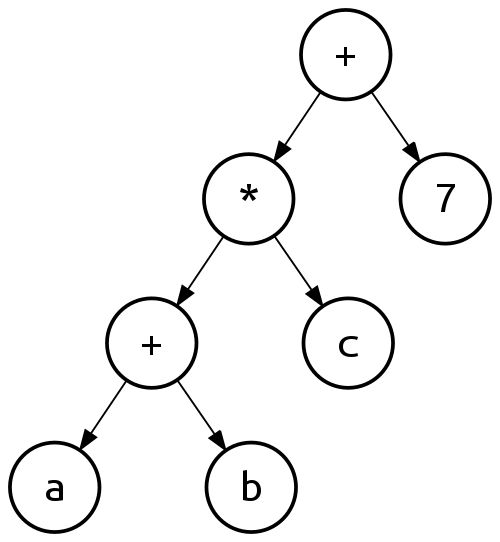
Figure 2: Example of binary expression tree. Figure taken from https://en.wikipedia.org/wiki/Binary_expression_tree

The expression tree approach allows to computationally work with symbolic equations - for example, to represent the equation \((a + b) \cdot c + 7 \cdot d\), simply add ’*’ and ‘d’ nodes to the ‘7’ node. In other words, expression trees also easily allow to change a given equation. This idea forms the core of genetic programming (GP), one of the most popular approaches to symbolic regression. Starting with a random population of these trees, GP randomly mutates the trees, conserving only the well-performing trees and repeat this until the convergence, analogous to how a population of genes evolves (Bongard and Lipson 2007; Schmidt and Lipson 2009; Maslyaev, Hvatov, and Kalyuzhnaya 2019). Alternatively, Petersen (2020) train a recurrent neural network to generate the trees corresponding to the unknown equations. A completely different approach to symbolic regression is taken by the team behind AI-Feynman (Udrescu and Tegmark 2019; Udrescu et al. 2020). They consider specifically equations originating from physics, and note that these equations often possess symmetry, separability or other various simplifying properties. By recursively applying these simplifications, the problem is split into a number of much easier to solve sub-problems, discovering a variety of seminal equations from physics. A final approach worth mentioning is that of the Bayesian model scientist (Guimerà et al. 2020). While the entire model space might be (infinitely) large, in practice many models and equations look alike or share much of their expression. Having mined all the equations on Wikipedia, the Bayesian model scientist generates various hypotheses for the form of the equation by combining fitting with this knowledge of all previous equations.

Symbolic regression is an active area of research, with the field seemingly focusing on discovering complex, explicit equations from synthetic, low-noise datasets (Udrescu and Tegmark 2019). However, most real, physical systems are governed by (coupled) differential equations, and the observations are noisy and sparse. Symbolic regression struggles in these settings, and as I will discuss later, the difficulty lies not in finding the equation, but in accurately calculating the features (i.e. the derivatives). An alternative approach based on sparse regression is much more for these systems and settings.

Sparse regression

Model discovery can be greatly simplified if we consider only differential equations - this doesn’t reduce the generality of our approach, as many physical systems are expressed as DEs. Considering again equation (1), note that it essentially is a linear combination of features, just like many other PDEs. This implies that many models can be written as,

\[\begin{align} \frac{\partial u}{\partial t} & = w_0 X_0 + \ldots + w_M X_M \\ & = w X^T \end{align}\]

I’m neglecting a huge group of models here: those with spatially or temporally varying coefficients! I’ll return to this issue in the next chapter.

where \(w_i\) is the coefficient corresponding to feature \(X_i\) and \(X\) the full feature matrix. Even within this restricted model space (i.e. the model is a linear combination of features), a combinatorial approach remains prohibitively expensive. However, by constructing a large set of possible features and combining these into a single matrix \(\Theta\), model discovery can be approached as a regression problem,

\[\begin{align} \tilde{w} = \min_w \left\lVert \frac{\partial u}{\partial t} - w \Theta \right\rVert^2. \end{align}\]

where \(\tilde{w}\) determines the model: \(\tilde{w}_i=0\) if feature \(i\) is not a part of the equation. More precisely, this has transformed model discovery into a variable selection problem; finding the correct model involves selecting the correct (i.e. non-zero) components of \(w\). The number of candidate terms \(N\) is typically much larger than the number of terms making up the equation \(M\), implying that most components of \(\tilde{w}\) should be zero. To promote such solutions, a sparsity promoting penalty is added - hence this approach is known as sparse regression. It was pioneered by Brunton, Proctor, and Kutz (2016) and has since become the de-facto method of performing model discovery.

Contributions

The sparse regression approach is elegant, flexible and widely applicable, but struggles on noisy and sparse data. When working with differential equations, the features making up the equation (\(\partial u / \partial t\) for both ODEs and PDEs and higher order spatial derivatives for PDEs) are not directly observed. Rather, the observed data \(u(x, t)\) must first be numerically differentiated to calculate the features. Numerical differentiation fundamentally is build on approximations, and when faced with sparse and noisy data it produces highly inaccurate results. This in turn fundamentally limits model discovery to low-noise, densely sampled datasets; if the features are corrupted, no approach will be able to select the right ones. As higher-order derivatives are more inaccurate, this issue specifically affects model discovery of PDEs, which often contains several higher-order spatial derivatives. If the calculation of the features is the limiting factor, this implies that model discovery should be approached as a distinct two-step process: calculating the features (step 1) is just as important, if not more, as selecting the right variables (step 2).

I’ll illustrate later how bad numerical differentiation really is.

Motivated by this line of reasoning, we realized that if our goal was to apply model discovery on experimental data, improving the accuracy of the features would have much more impact than constructing more robust sparse regression algorithms. A common approach to improve the accuracy of the features is to approximate the data using some data-driven model, for example using polynomials or a fourier series, and perform sparse regression based on the features calculated from that approximation. My work is build on the idea that by integrating these two steps, model discovery can be made much more robust: the approximation makes it easier to discover the governing equation, while this equation in turn can be used to improve the approximation. In other words, I argue that data-driven and first-principle modelling are not opposites, but that they can mutually improve each other. Specifically, my work focuses on 1) constructing accurate representations of (noisy) data using neural networks and 2) how to incorporate the knowledge of the governing equation back into these networks. Our overarching goal was to improve model discovery of partial differential equations on noisy and sparse datasets, opening the way for use on real, experimental datasets.

More generally put, data-driven modelling improves first-principle modelling by yielding providing better features, while first-principle modelling improves data-driven modelling by infusing it with physical biases.

In Both et al. (2019) we show that such neural networks significantly improve the robustness of model discovery compared to unconstrained neural networks or classical approaches. Improving on this, in Both, Vermarien, and Kusters (2021) we present a modular framework, showing how these constrained networks can utilize any sparse regression algorithm and how to iteratively apply the sparse regression step, boosting performance further. In our latest work (Both and Kusters 2021), we build upon the first two articles to construct a fully differentiable model discovery algorithm by combining multitask learning and Sparse Bayesian Learning. Besides these methodological papers, we show in Both, Tod, and Kusters (2021) that neural network based model discovery needs much less samples to find the underlying equation when they are randomly sampled, as opposed to on a grid. This marks a fundamental difference with classical approaches, which struggle with off-grid sampled data. In Both and Kusters (2019) we introduce Conditional Normalizing Flows. CNFs allow to learn a fully flexible, time-dependent probability distribution, for example to construct the density of single particle data. In Both and Kusters (2021) we build on this to discover a population model directly from single particle data. This series of articles was released under the name DeepMoD - Deep Learning based Model Discovery. Most of this work is collected in an open-source software package called DeePyMoD. Taken together, our work strongly establishes the argument for neural network based surrogates, constrained by the underlying physics, for model discovery on real, experimental data.

I’ve worked on several other topics, but I have chosen to focus on my main projects.

Organization of this thesis

I’ve written my thesis using Distill for R Markdown, a format based on the excellent online journal Distill. Distills typesetting and typography is strongly based on the Tufte style and is optimized for digital viewing: I’ve included some interactive plots, and hover over footnotes to see their content³ or over citations to see the full one - often with a link to an Arxiv version (Both and Kusters 2021). All this means that while you can read it on paper, you will miss out on these features, so I highly recommend using this website.

Distill has an excellent article discussing the uses of interactive articles.

This thesis itself is also a small experiment. Instead of writing a long static document which is likely to only be read by the committee, can I write something a little more modern which will be useful to others, perhaps those not familiar with the field? Instead of writing a comprehensive review examining all the papers in the field, can I write something which gives a broader overview, discusses key papers in-depth and introduce the key challenges? The website in front of you is the answer I came up with.

• I have split the background of my work into two pages: Regression shortly discusses the regression approach to model discovery and presents the key papers of the field. As I argue in this thesis, surrogates should be a key component of model discovery algorithms. In Surrogates I discuss various classical approaches, but will spend the bulk of the chapter on Physics Informed Neural Networks (PINNs).
• DeepMoD is the umbrella under which I’ve collected all of my work done during my PhD on model discovery from January 2019 until July 2021. I start by explaining the main idea behind our approach, and then summarize our papers and list their respective contributions.
• In Discussion I reflect on our work and put it in context. Finally, I consider the open questions and challenges for model discovery.

Each chapter article can be read on its own, but I suggest following the order in which I’ve introduced them above. I hope this thesis is able to convey all that I’ve learned and done the last few years - happy reading!

Acknowledgements

---

1. This term is mostly used by natural scientists working on physical datasets. Several other terms are in use, depending on the field and the exact goal. In engineering, it is often referred to as system identification, while in machine learning it is often known as causal inference.↩︎

2. In this setting also often referred to as dynamical systems.↩︎

3. No more scrolling!↩︎