Sparse regression for model discovery

The de-facto method of model discovery on differential equations is to use sparse regression. In this chapter I discuss this approach and various sparsity-promoting techniques. Sparse regression is widely applicable and has been extended along multiple axes. I review the key extensions and shortly consider the alternatives.

Figure 1: One-dimensional solution of the Kuramoto-Shivashinsky equation.

Consider again the Kuramoto-Shivashinsky equation,

\[\begin{align} \frac{\partial u}{\partial t} = \frac{\partial^2 u}{\partial x^2} - \frac{\partial^4 u}{\partial x^4} - u \frac{\partial u}{\partial x}. \tag{1} \end{align}\]

It is a fourth order, non-linear partial differential equation giving rise to the beautifully rich behaviour of figure 1. This complexity - a fairly unusual fourth-order derivative and a non-linear term - also poses a challenge for model discovery. Is it really possible to discover an equation this complex autonomously from data? In this chapter I introduce how sparse regression makes this possible, using the Kuramoto-Shivashinksy equation as an example. Before reviewing regression and various sparsity-promoting regularizations, I shortly consider why the sparse regression technique can be used. This chapter ends with an overview of the key extensions which have been developed.

For more information on the KS equation, see Wikipedia or Encyclopedia of Math.

Structure of differential equations

While the Kuramoto-Shivashinksy equation appears complex, its structure is not particularly unique. In fact, it shares many features with other models. Consider for example the Cahn-Hilliard equation, which describes phase separation of a fluid with concentration \(c\), diffusion coefficient \(D\) and a length scale \(\sqrt{\gamma}\):

\[\begin{align} \frac{\partial c}{\partial t} = D \nabla^2\left(c^3 - c- \gamma \nabla^2 c\right), \end{align}\]

or the Korteweg-de Vries equation, which describes the speed \(u\) of waves in shallow water,

\[\begin{align} \frac{\partial u}{\partial t} = -\frac{\partial^3 u}{\partial x^3} + 6 u\frac{\partial u}{\partial x}. \end{align}\]

All three equations describe completely different systems, but share a similar structure: each consists of 1) a linear combination of 2) relatively simple features¹. Indeed, considering the list of non-linear partial differential equations on Wikipedia, only very few equations have features composed of more than two terms, such as \(u \cdot u_{x} \cdot u_{xxx}\). Property 2 implies that most models can be constructed from a small, finite set of elements consisting of,

An interesting question is if this is a fundamental fact or a consequence of our approach to physics.

1. Polynomials of the observable \(u\) up to order \(p\): \(1, u, u^2, \ldots\).
2. Derivatives up to order \(q\): \(u_{x}, u_{xx}, u_{xxx}, \ldots\)
3. Combinations of these two features: \(u \cdot u_x, u^2 \cdot u_{xxx}, \ldots\)

For most known equations, \(p \leq 3\) and \(q \leq 4\), typically yielding 20-30 candidate features. Even at this size, a combinatorial search is computationally too expensive, as it involves solving the PDE. However, by exploiting property 1, i.e. that the unknown equation is a linear combination of the candidate features, model discovery can be expressed as a regression problem.

I’m only considering non-coupled, one-dimensional cases here, but the argumentation extends to higher dimensions. The library size will be much bigger, and the combinatorial search will be even more expensive, but most features will still be a combination of two components.

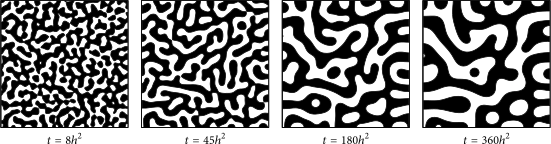
Figure 2: Solution of the Cahn-Hilliard equation. Image taken from https://www.hindawi.com/journals/mpe/2016/9532608/

Regression for model discovery

Expressing model discovery as a regression problem starts by combining all \(M\) candidate features into a single library matrix \(\Theta\),

\[\begin{align} \Theta = \begin{bmatrix} \vert & \vert & \vert & \vert & \vert\\ 1 & u & u_x & \ldots & u^2u_{xx}\\ \vert & \vert & \vert & \vert & \vert \end{bmatrix} \end{align}\]

i.e. each column of \(\Theta \in \mathcal{R}^{N \times M}\) contains a single feature. Assuming the equation is a linear combination of these features, the unknown equation can be written as,

\[\begin{align} \frac{\partial u}{\partial t} = \Theta \xi \tag{2} \end{align}\]

where \(\frac{\partial u}{\partial t} \in \mathcal{R}^N\) is the time derivative and \(\xi \in \mathcal{R}^{M}\) the coefficient vector describing the equation. If a component \(\xi_j\) is zero, the corresponding feature \(\Theta_j\) is not a part of the equation, and vice versa. For example, if \(\Theta = \begin{bmatrix} 1 & u & u_{x} & uu_{x} \end{bmatrix}\),

\[\begin{align} \xi = \begin{bmatrix} 0.0 & 0.5 & 0.0 & -2.0 \end{bmatrix}^T \end{align}\]

corresponds to the equation

\[\begin{align} \frac{\partial u}{\partial t} = \frac{1}{2} u - 2 \frac{\partial^2 u}{\partial x^2}. \end{align}\]

With eq. (2), instead of comparing all models which can be build with the candidate features, now we only need to find a single vector \(\xi\) by minimizing,

The way I like to think about this, is that with this approach we’re essentially fitting all models at the same time.

\[\begin{align} \hat{\xi} = \min_\xi\left\lVert u_t - \Theta \xi \right\rVert_2^2 \tag{3} \end{align}\]

This least-squares problem is trivial to solve,² but will, unfortunately, not yield the correct result in most cases. Since the number of features \(M\) is likely to be much larger than the number of terms making up the unknown equation, solving eq. (3) will overfit the model: very little if any components of \(\hat{\xi}\) will be zero. Luckily, equation (3) can be adapted to yield results \(\hat{\xi}\) win which many components are exactly 0, a property known as sparsity. This is known as sparse regression and this approach to model discovery was pioneered by Brunton, Proctor, and Kutz (2016) for ODEs and extended to PDEs in S. H. Rudy et al. (2017) . Various ways to promote the sparsity of solutions to eq. (3) exist, and I discuss those in the next section.

Technically this norm is only appropriate for Gaussian, white noise (i.e. zero-mean, uncorrelated). Extensions to other noise models are called generalized linear models, but in practice only white noise is used.

Regularized regression

To promote sparsity of the resulting vector, we augment the objective function eq. (3) with a regularization function \(R(\xi)\) on the unknown coefficients \(\xi\),

\[\begin{align} \hat{\xi} = \min_{\xi} \frac{1}{N}\left\lVert u_t - \Theta \xi \right\Vert_2^2 + \lambda R(\xi) \tag{4} \end{align}\]

where \(\lambda\) sets the strength of the regularization. The choice of \(R(\xi)\) affects which behaviour is penalized. Three common choices are,

The \(1/N\) factor is not strict required, but has the benefit of making the regularization strength \(\lambda\) sample size-independent.

• \(R(\xi) = \left\lVert \xi \right\rVert_0\), also known as \(\ell_0\) regularization, penalizes the number of non-zero components, promoting sparsity in the final solution.
• \(R(\xi) = \left\lVert \xi \right\rVert_1\), known as \(\ell_1\) regularization, penalizes the magnitude of \(\xi\) linearly, also promoting sparsity in the final solution.
• \(R(\xi) = \left\lVert \xi \right\rVert_2^2\), also called \(\ell_2\) regularization, penalizes the magnitude of \(\xi\) quadratically, preventing large magnitude coefficiens in the final solution.

These penalties can also be combined: for example, the elastic net (Zou and Hastie 2005) combines the benefits of both \(\ell_1\) and \(\ell_2\) regularization by defining

\[\begin{align} R(\xi) = \alpha \left\lVert \xi \right\rVert_1 + (1-\alpha)\left\lVert \xi \right\rVert_2^2. \end{align}\]

Since these regularizations are central to sparse regression and model discovery, I want to discuss each of these three regularizations in-depth.

More generally, \(\xi\) can be penalized by any \(p\)-norm, but in practice only \(p=1, 2\) are used.

Figure 3: Penalty functions of \(\ell_0, \ell_1\) and \(\ell_2\) regularization.

\(\ell_0\)

\(\ell_0\) regularization penalizes the number of non-zero components through the penalty function,

\[\begin{align} \left\lVert \xi \right \rVert_0 = \sum_j \xi_j^*, \quad \xi_j^* = \begin{cases} 1 & \text{if $\xi_j \neq 0$}\\ 0 & \text{if $\xi_j = 0$} \end{cases} \end{align}\]

This makes it an obvious choice for promoting sparsity: if the amount of terms is penalized, solutions with fewer terms are favoured, and additionally, it does not affect the magnitude of the components, making it an unbiased estimator. Unfortunately, by penalizing the number of terms (also known as the support) the objective function becomes non-differentiable and non-convex. Simply put, this regularization still effectively involves solving a combinatorial problem. Maddu et al. (2019) show that an approximation known as Iterative Hard Thresholding can be an effective method in model discovery. A different avenue of research tackles these issues head-on by taking a probabilistic approach. For example, Louizos, Welling, and Kingma (2018) consider the penalty as the sum of Bernouilli random variables, allowing gradient-based optimization. Nonetheless, these approaches are still computationally expensive.

\(\ell_1\) - Lasso

Given these issues, a common approach is to relax the problem and apply \(\ell_1\) regularization,

\[\begin{align} \left \lVert \xi \right \rVert_1 = \sum_j \left\lvert \xi_j \right\rvert. \end{align}\]

Compared to an \(\ell_0\) regularized problem, this too yields sparse solutions (I will discuss why it does later on), but is convex and can be efficiently solved using proximal method such as FISTA (Beck and Teboulle 2009), despite its non-differentiability at \(x=0\). Usually this approach is called Lasso (Least Absolute Shrinkage and Selection operator), as it the sparsest norm still yielding a convex problem (Tibshirani 2011).

The Lasso is a popular approach when sparsity is required, but it does not come without its drawbacks. It yields a biased estimate of the coefficients, but a more significant issue is that it is not guaranteed to be consistent³. An estimator is consistent if the estimate approaches the true value with increasing sample size:

\[\begin{align} \tag*{(Consistency)} \hat{\xi} \to \xi_{\text{true}} \quad \text{as $N \to \infty$} \end{align}\]

While this might seem like a trivial point, its implications are not: an inconsistent estimator will not be able to recover the truth, even with an infinite number of samples. The Lasso is consistent only if the Irrepresentable condition (IRC) is satisifed (Zhao and Yu, n.d.). In practice the IRC is often violated, implying the Lasso is unable to recover the ground truth. The violation is caused by correlation between variables, and the lasso can be made consistent by scaling the components in the penalty. For example, the adaptive Lasso (Zou 2006) scales the penalty as

\[\begin{align} \tag*{(Adaptive Lasso)} \sum_j w_j \left\lvert \xi_j \right\rvert \end{align}\]

where \(w_j = 1 / \left\lvert \xi_j^* \right \rvert^\gamma\), with \(\xi_j^*\) the result of a different consistent estimator and \(\gamma\) a scaling factor.

\(\ell_2\) - Ridge

The third popular regularization is an \(\ell_2\) penalty,

\[\begin{align} \tag*{(Ridge)} \sum_j \left\lvert \xi_j\right\rvert^2, \end{align}\]

also known as ridge regression. Ridge regression can be analytically solved, thus having essentially the same computational cost as least squares,⁴ and can handle highly correlated variables. Unfortunately, ridge regression favours results where none of the coefficients are large, but not exactly zero either - in other words, it does not yield a sparse coefficient vector. To see why Lasso yields sparse results while ridge regression does not, consider figure 4. The ovals show the level sets of the loss due the fitting term (i.e. the first term of eq. (4)) and the loss due the regularization is represented by the circle (ridge) and square (lasso). The solution of the regularized problem is the intersection of these two losses. For the \(\ell_1\) regularization, the intersection happens at the corners, leading to sparse coefficients, whereas for the \(\ell_2\) regularization it happens in the middle, yielding small but non-zero coefficients. Model discovery often relies on heuristics and some approaches based on ridge regression show good performance, despite it not mathematically yielding sparse coefficients. For example, SINDy (Brunton, Proctor, and Kutz 2016), one of the most popular model discovery approaches, uses ridge regression.

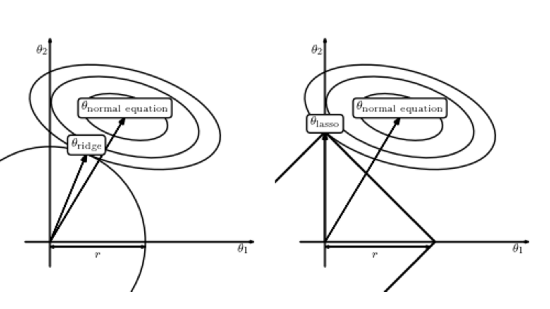
Figure 4: Comparison of Lasso and Ridge losses. Figure from https://www.astroml.org/book_figures/chapter8/fig_lasso_ridge.html

Heuristics

Besides these regularizations, various other heuristic are often applied to improve the sparsity of the obtained coefficients. I discuss two commonly used ones: thresholding and sequential regression.

Thresholding

It is quite common that we recover a sparse vector which is approximately right: the required terms stand out, but several other small but non-zero components exist, despite regularization. Performance can be strongly improved by thresholding this sparse vector. Since all components have different dimensions, the features are first normalised by their \(\ell_2\) norm,

\[\begin{align} \Theta_j^* =\frac{\Theta_j}{\left\lVert \Theta_j \right\rVert_2}, \end{align}\]

allowing us to define normalized coefficients as,

\[\begin{align} \xi_j^* = \xi_j \cdot \left\lVert\Theta_j\right\rVert_2. \end{align}\]

We can also normalize the target vector, i.e. the time derivative, to make everything dimensionless.

Given some threshold value \(\eta\), the threshold operation is then defined as

\[\begin{align} \xi_j = \begin{cases} \xi_j & \text{if $\xi^*_j \geq \eta$}\\ 0 & \text{if $\xi^*_j < \eta$} \end{cases} \end{align}\]

The value of \(\eta\) is usually preset (i.e. a hyperparameter), but it can also be learned (S. H. Rudy et al. 2017).

Sequential regression

A second trick is to sequentially refine the estimate by iteratively performing sparse regression on only the active features selected by the previous estimator,

\[\begin{align} \xi^{i+1} = \min_{\xi_i} \frac{1}{N}\left\lVert u_t - \Theta^i \xi^i \right\Vert_2^2 + \lambda R(\xi^i) \\ \Theta^{i+1} = \Theta^i[\xi^{i+1} \neq 0] \end{align}\]

until \(\xi\) converges. While this does bias the results as coefficients can only be removed, not added, in practice it works well.

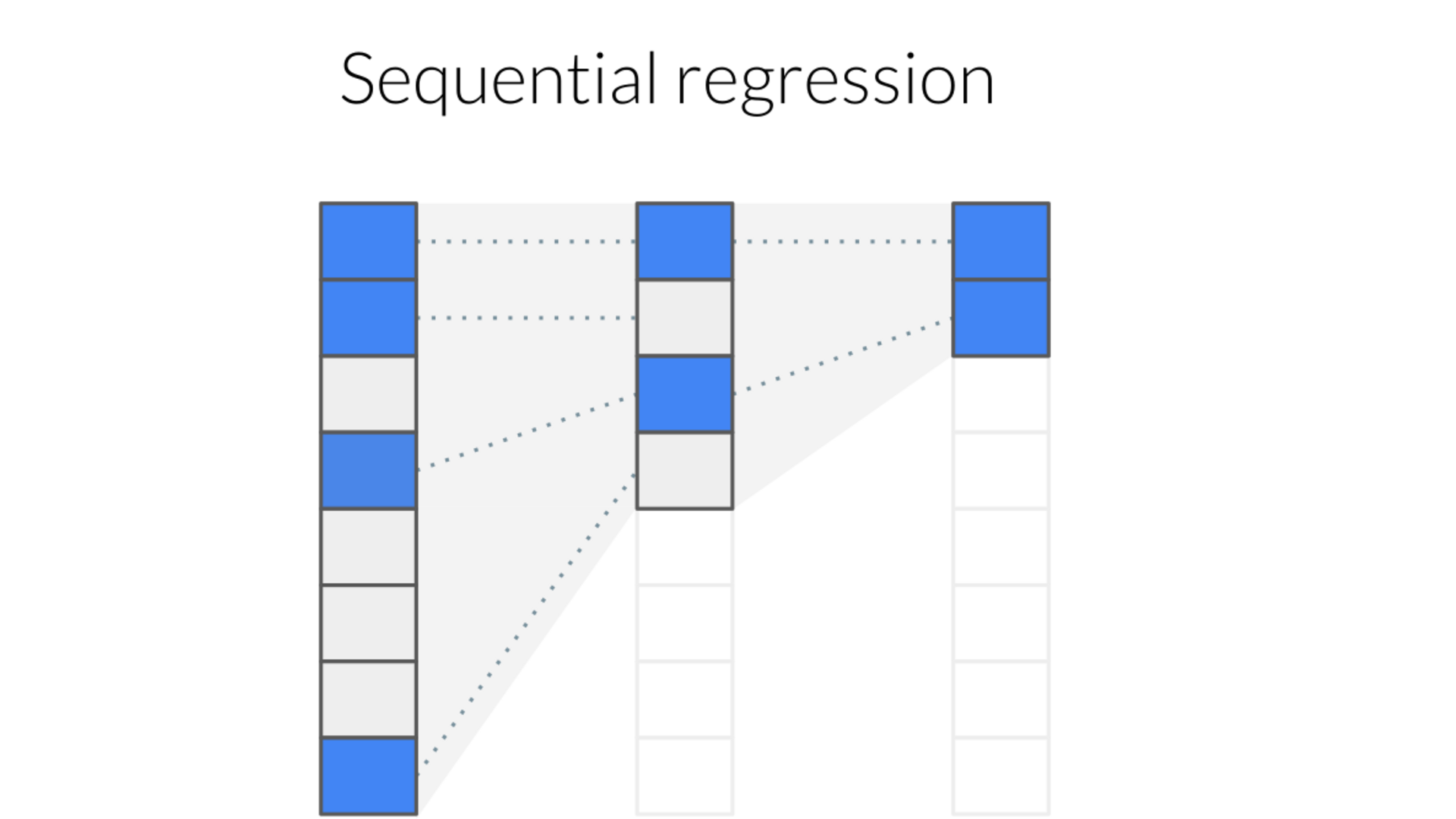
Figure 5: Illustration of sequential regression.

Extensions

Sparse regression forms a very flexible and general approach to model discovery and has been adapted, extended and improved in various ways since its introduction. In the next section I discuss the key papers which have either solved important open questions, or make significant progress towards it.

Stability selection

In the previous section we considered the effect of different regularizations on sparsity. An additional important factor is the strength of this regularization, denoted by the factor \(\lambda\) in eq. (4). Figure 6 shows the solution \(\hat{\xi}\) as a function of the regularization strength \(\lambda\). The resulting sparse vector is strongly dependent on \(\lambda\); the lower the amount of regularization, the more features are selected.

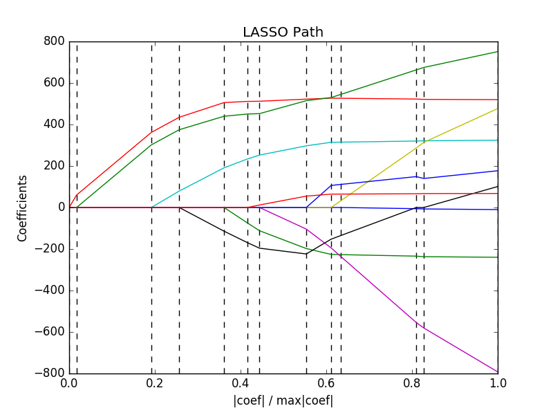
Figure 6: Lasso path. Figure from https://scikit-learn.org/0.18/auto_examples/linear_model/plot_lasso_lars.html

The default method to choose hyper-parameters such as \(\lambda\) is cross-validation (CV). CV consists of splitting the data into \(k\) folds⁵, training the model on \(k-1\) folds and testing model performance on the remaining fold. This process is repeated for all folds and averaging over the results yields a data efficient but computationally expensive approach to hyperparameter tuning. CV optimizes for predictive performance - how well does the model predict unseen data? -, but model discovery is interested in finding the underlying structure of the model. Optimizing for predictive performance might not be optimal; a correct model certainly generalizes well, but optimizing for it on noisy data will likely bias the estimator to include additional, spurious, terms. An alternative metric which optimizes for variable selection is stability selection (Meinshausen and Buehlmann 2009).

The key idea is that while a single fit probably will not be able to discriminate between required and unnecessary terms we expect that among multiple fits on sub-sampled datasets the required terms will consistently be non-zero. Contrarily, the unnecessary terms are essentially modelling the error and noise, and will likely be different for each subsample. More specifically, stability selection bootstraps a dataset of size \(N\) into \(M\) subsets \(I_M\) of \(N/2\) samples, and defines the selection probability \(\Pi^\lambda_j\) as the fraction of subsamples in which a term \(j\) is non-zero

\[\begin{align} \Pi^\lambda_j = \frac{1}{M}\sum_M \mathcal{1}(j \in S^\lambda(I_M)) \end{align}\]

where \(S^\lambda_j\) is the recovered support, i.e. whether a term is non-zero. The support can be determined using any sparse regression method: Meinshausen and Buehlmann (2009) use Lasso, but Maddu et al. (2019) use a relaxed \(\ell_0\) penalty. Calculating the selection probability for a range of regularization strengths \(\Lambda\) yields the stability path (figure 7).

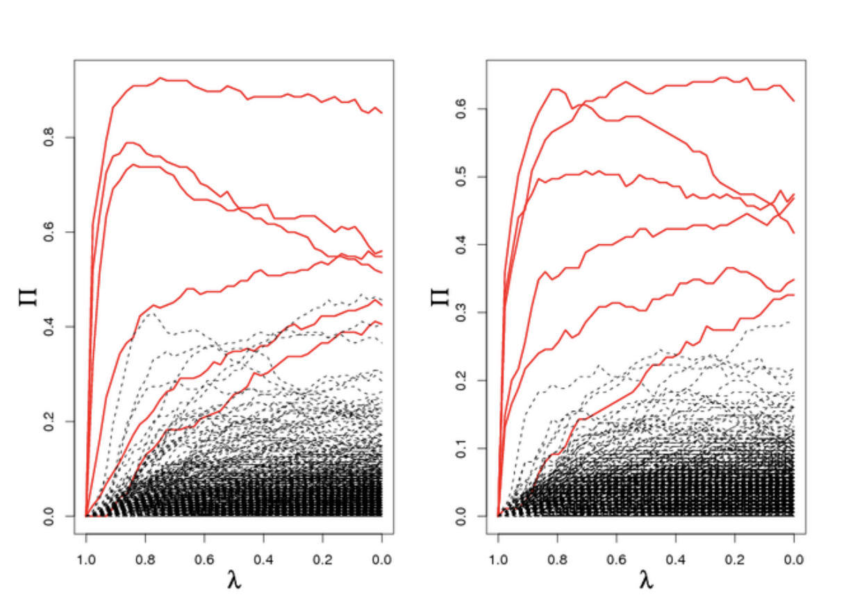
Figure 7: Stability paths. Figure from https://thuijskens.github.io/2018/07/25/stability-selection/

Using the stability path, the final support is determined by selecting all components with a selection probability above a given threshold \(\pi_{\text{thr}}\),

\[\begin{align} S^{\text{stable}} = \{j: \max_{\lambda \in \Lambda} \Pi_j^\lambda > \pi_{\text{thr}}\} \end{align}\]

As the active components are determined from a range of \(\lambda\), stability selection does not require making a point estimate for the regularization strength as with CV. Stability selection has been shown to outperform cross validation in model discovery, especially at higher noise levels (Maddu et al. 2019, 2020).

Multi-experiment datasets

A dataset rarely consists of a single experiment - they are comprised of several experiments, each with different parameters, initial and boundary conditions. Despite these variations, they all share the same underlying dynamics. To apply model discovery on these datasets we need a mechanism to exchange information about the underlying equation among the experiments. Specifically, we need to introduce and apply the constraint that all experiments share the same support (i.e. which terms are non-zero).

Consider \(k\) experiments, all taken from the same system, \(\{\Theta \in \mathcal{R}^{N \times M} , u_t \in \mathcal{R}^{N}\}_k\), with an unknown sparse coefficient vector \(\xi \in \mathcal{R}^{M \times k}\). Applying sparse regression on each experiment separately is likely violate this constraint; while it will yield a sparse solution for each experiment, the support will not be the same (see figure 8). Instead of penalizing single coefficients, we must penalize groups - an idea known as group lasso⁶ (Huang and Zhang 2009). Group lasso first calculates a norm over all members in each group (typically an \(\ell_2\) norm), and then applies an \(\ell_1\) norm over these group-norms (see figure 8),

\[\begin{align} \tag*{Group sparsity} R(\xi) = \sum_{j=1}^{k} \left | \sqrt{\sum_{i=1}^{M} \left\lvert \xi_{ij}\right \rvert^2}\right | \end{align}\]

This approach drives groups of coefficients to zero, rather than single coefficients, and thus satisfies the constraint (see figure 8). Group sparsity has been successfully used for model discovery on multiple experiments (Silva et al. 2019), or with space- or time-dependent coefficients (see next section), but can also be exploited to impose symmetry (Maddu et al. 2020).

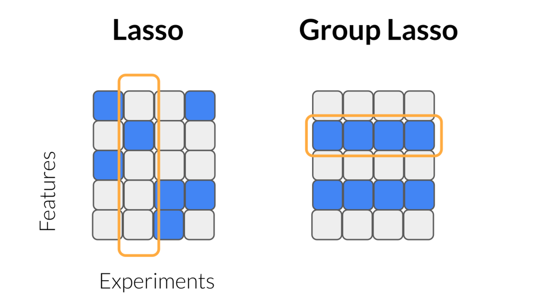
Figure 8: Lasso applies the penalty vertically, while group lasso applies the penalty horizontally.

Time/space dependent coefficients

So far we have implicitly assumed that all the governing equations have fixed coefficients. This places a very strong limit on the applicability of model discovery; usually coefficients are fields depending on space or time (or even both!), so that \(\xi = \xi(x, t)\). As a first attempt at solving this, S. Rudy et al. (2018) learn the spatial or temporal dependence of \(\xi\) by considering each corresponding slice as a separate experiment with different coefficients, and applying the group sparsity approach we introduced in the previous section. A Bayesian version of this approach was studied by Chen and Lin (2021). It is important to note that in both these works \(\xi(x, t)\) is not parametrized; it is not the functional form which is inferred, but simply its values at the locations of the samples.

A interesting approach not based on sparse regression is taken by Long, Lu, and Dong (2019) . They note that since derivatives can be approximated as a convolution, learnable filters can be used to discover the underlying equation, even with spatially varying sources.

Information-theoretic approaches

The sparse regression approach tacitly assumes that the sparsest equation is also the correct one. While not an unreasonable assumption, it does require some extra nuance, as there often is not a single correct model. Many (effective) models are constructed as approximations of a certain order depending on the accuracy required. A first order approximation yields the sparsest equation, while the second order model could describe the model better. Another example is that a system can be locally modelled by a simpler, sparser equation. In both cases neither model is incorrect - they simply make a different trade-off. Information-theoretic approaches give a principled way to balance sparsity of the solution with accuracy.

Consider two models \(A\) and \(B\), each with likelihood \(\mathcal{L}_{A, B}\) and \(k_{A, B}\) terms. Model B has a higher likelihood, \(\mathcal{L}_B > \mathcal{L}_A\), indicating a better fit to the data, but also consists of more terms, \(k_B > k_A\). The Bayesian Information Criterion (BIC) and the closely related Akaike Information Criterion (AIC) are two metrics to decide which balance these two objectives,

\[\begin{align} \text{BIC} = k \ln n - 2 \ln \mathcal{L} \end{align}\] and the Akaike Information Criterion, \[\begin{align} \text{AIC} = 2k- 2 \ln \mathcal{L}. \end{align}\]

If model \(B\) has a lower AIC or BIC than model \(A\) it is a better, even if \(k_B > k_A\). In other words, these criteria give a principled way to decide the trade-off between how well the model fits fits the data and the complexity of the model. This approach has been used by Mangan et al. (2017) to decide between various discovered models, and a similar approach based on minimum description length was used by Udrescu and Tegmark (2019) .

As we discussed, it is likely for multiple models to be correct simultaneously, all with similar BIC or AIC. Each of these models is essentially the model best describing the data at a certain accuracy, and all of the models together describe a curve in model space known as the Pareto Frontier. All models on this curve are correct, but of varying complexity, and we merely need to pick the model corresponding to the accuracy to which we wish to describe the data (Udrescu et al. 2020).

Pareto optimality is a very wide applicable concept, as it essentially describes how to make the trade-off between multiple conflicting objectives.

Bayesian approaches

The requirement that the resulting coefficient vector \(\xi\) be sparse is essentially a form of prior knowledge. A principled way to include such prior knowledge is given by Bayes’ theorem, which states for some data \(X\) and parameters \(w\)

\[\begin{equation} \overbrace{p(w \mid X)}^{\text{posterior}} = \frac{\overbrace{p(X \mid w)}^{\text{likelihood}}\ \overbrace{p(w)}^{\text{prior}}}{p(X)}. \end{equation}\]

The likelihood describes the probability of the data \(X\) for a given parameter \(w\), while the prior describes the probability distribution of the parameter \(w\). The posterior then is the distribution of \(w\) given the data and the prior. Contrary to maximum likelihood approaches which yield point estimates, Bayesian approaches yield distributions, allowing to quantify uncertainty. Additionally, the inclusion of the prior effectively regularizes the problem, making Bayesian regression typically much more robust than MLE approaches.

The sparsity of \(\xi\) can be encoded in the prior in various ways. A common approach known as Sparse Bayesian Learning (Tipping 2001) takes a zero-centred Gaussian as prior,

\[\begin{align} p(\xi_j \mid \alpha_j) = \mathcal{N}(w_i \mid 0 , \alpha_j^{-1}). \end{align}\]

The SBL assumes all terms are zero, but the confidence of that decision (\(\alpha_j\)) is inferred from data. As \(\alpha_j \to \infty\), the prior becomes infinitely sharp at zero, and the component is pruned from the model. The Gaussian prior is not particularly sparse, but Yuan et al. (2019) nonetheless show good performance with model discovery. Sparsity can be more strongly promoted by using a Laplacian prior to yield a Bayesian Lasso (Helgøy and Li 2020), or a so-called spike-and-slab-prior (Nayek et al. 2020).

The field of Bayesian approaches to model selection is so rich it deserves a book on its own. I restrict myself here mainly to some approaches used in the model discovery of PDEs.

---

1. Although they all share a diffusive term - we can’t seem to escape entropy.↩︎

2. It has an analytical solution but for numerical stability one often uses QR decomposition or SVD. Addtionally, least squares is a so-called BLUE - which means that the estimate \(\hat{\xi}\) is unbiased and has the lowest variance as long as the errors are uncorrelated.↩︎

3. In literature this sometimes also referred to as the oracle property.↩︎

4. Simply add \(\sqrt{\lambda}\) along the diagonal of the gram matrix, or augment the data and solve it like a standard least squares problem↩︎

5. subsets↩︎

6. Technically this is group sparsity, but since almost always lasso is used, these terms are used interchangeably.↩︎