Differentiation & Surrogates

The sparse regression approach to model discovery discovers equations from a large set of candidate features. When discovering PDEs, many of these features are comprised of (higher-order) derivatives, which are challenging to calculate accurately. In this chapter I illustrate the effect of numerical differentiation on model discovery, motivating the use of surrogate models. These models mimic the observed data, but yield much more accurate derivatives. I discuss some often-used surrogates and show why (constrained) neural networks make excellent surrogates.

Surrogates¹ are a widely used approach to approximate a dataset or model by a different, data-driven model with certain desirable properties. For example, a computationally cheap surrogate can be used to replace a computationally expensive simulation, or an easily-differentiable surrogate can be used to approximate a dataset we wish to differentiate. I discuss various surrogates used in the model discovery community and make the case for neural networks as surrogates. A neural network-based surrogate can be strongly improved by constraining it to the underlying physics using an approach known as Physics Informed Neural Networks (PINNs), and I end the chapter with a short introduction to Normalizing Flows (NFs). Before all of this though, I want to discuss why surrogates are needed in model discovery.

The need for surrogates

Using the sparse regression approach to discover PDEs requires calculating various higher-order derivatives. For example, a diffusive term is given by a second order derivative, \(\nabla^2 u\), while the Kuramoto-Shivashinksy equation requires a fourth order derivative. Consider the definition of the derivative, \[\begin{align} \frac{du}{dx} = \lim_{h\to 0}\frac{u(x + h) - u(x)}{h}. \end{align}\] Since data is always sampled at a finite spacing, in practice a derivative must always be approximated,

\[\begin{align} \frac{du}{dx} \approx \frac{u(x + h) - u(x)}{h}. \tag{1} \end{align}\]

This equation forms the basis of numerical differentiation. In what follows we assume the data has been sampled on a grid with spacing \(\Delta x\), allowing the use of a more natural notation in terms of grid index \(i\). Equation (1) takes into account only the ‘following’ sample \(u_{i+1}\) at position \(+h\) and is hence known as a forward-difference scheme. A more accurate estimate can be obtained by taking into account both the previous sample \(u_{i-1}\) and following sample \(u_{i+1}\), yielding the popular second-order central difference scheme,

Actually, we can exactly calculate the derivative, but the trade-off is that we need to approximate the data using some other model - a surrogate!

\[\begin{align} \frac{du_i}{dx} \approx \frac{u_{i+1} - u_{i-1}}{2 \Delta x}. \tag{2} \end{align}\]

Applying eq. (2) recursively yields higher order derivatives,

\[\begin{align} \frac{d^2u_i}{dx^2} \approx \frac{u_{i-1} - 2u_i + u_{i+1}}{\Delta x^2} \\ \frac{d^3u_i}{dx^3} \approx \frac{-u_{i-2} + 2 u_{i-1} - 2 u_{i+1} + u_{i+2}}{2\Delta x^3} \tag{3} \end{align}\]

Numerical differentiation through finite differences has various attractive properties: it’s easy to implement and computationally cheap. However, these advantages come with large drawbacks:

• The approximation is only valid for small \(\Delta x\). If the samples are spaced far apart, the resulting derivative will be inaccurate. Higher order schemes can alleviate this only slightly.
• Higher order derivatives are calculated by successively applying the approximation (see (3)). Consequently, small errors in lower orders get propagated and amplified to higher orders, making estimates of these higher-order derivatives highly inaccurate.
• At the edges of the dataset (e.g. \(u_0\)), the derivatives cannot be calculated. Doing so would require extrapolating, which is highly inaccurate, so typically the data at the edge is simply discarded. Since higher order derivatives utilize large stencils, this can amount to a significant part of the data when working with small datasets.

However, the dominant issue is numerical differentiation’s inability to deal with noisy data. Even low noise levels of i.i.d. white noise (<10%) can corrupt the features to such an amount that model discovery becomes impossible. We illustrate these issues in figure 1, where we show with a toy function \(f(x) = cos(x^2)\) the effect of data sparsity and 10% applied noise on the first and third derivative. Note that while the effect on the first derivative is still relatively limited, the third derivative is strongly corrupted. For the sparse data we can still qualitatively observe the behaviour, albeit with much lower peaks, but the noise has corrupted the data almost completely.

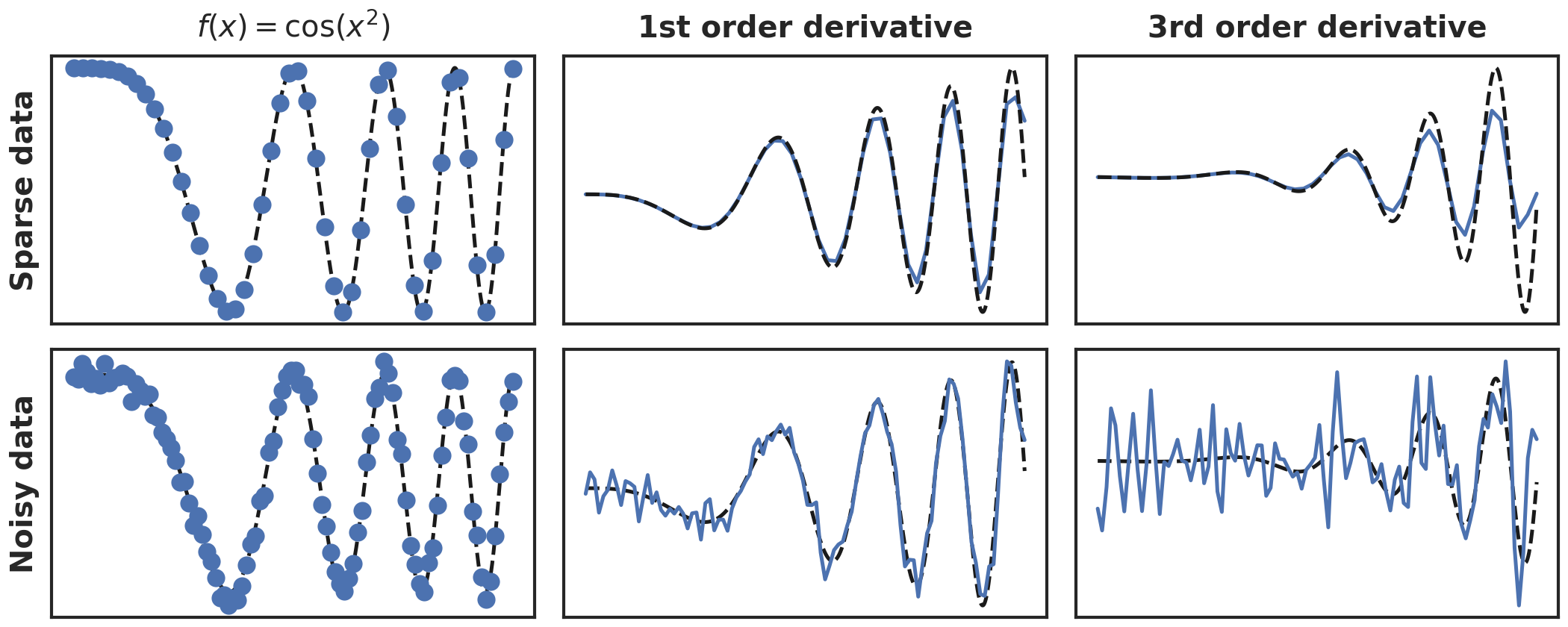
Figure 1: Numerical differentiation of noisy and sparse data. Blue are the samples, black dashed line the ground truth.

Denoising the to-be-differentiated data and regularizing the differentiation process increases accuracy (Van Breugel, Kutz, and Brunton 2020), but remains inadequate for very noisy data. Luckily, surrogates offer a way out. By fitting an easily-differentiable model such as a polynomial to the data, the problem of numerical differentiation is circumvented; the derivative of a polynomial can be trivially calculated symbolically. This does not mean that calculating the features is easy; the difficulty of determining the derivatives is now displaced to the task of accurately fitting the surrogate model the noisy data. In the next section I discuss the surrogate models which are often used in model discovery.

Surrogates: local versus global

Model discovery requires surrogates to be easily differentiable, but also to be flexible. The surrogate model must be able to accurately model the data: given some data \(u(x)\), the surrogate \(p(x)\) ought to have enough degrees of freedom to approximate \(u\) reasonably, i.e. \(p(x) \approx u(x)\). A classical approach is to represent \(p(x)\) as a series expansion,

Note that the surrogate model doesn’t need to be interpretable - we’re merely trying to represent and interpolate the data in such a a way that we can easily take derivatives.

\[\begin{align} p(x) = \sum_n a_n h_n(x) \end{align}\] where \(a_n\) are picked such that \(p(x) \approx u(x)\). The derivatives are now easily (and accurately!) calculated - it’s simply the sum over the derivatives of the basis functions: \[\begin{align} \frac{du}{dx} \approx \frac{dp(x)}{dx} = \sum_i a_i \frac{dh_i(x)}{dx} \end{align}\] The flexibility of the surrogate strongly depends on the choice of basis functions. A choice well-known to physicists is to use the Fourier basis, \[\begin{align} h_n(x) = e^{2 \pi i n x}. \end{align}\] Using Fourier series has several attractive properties: they’re computationally efficient, well established, and are particularly useful for calculating derivatives. The fourier transform of a \(p\)th order derivative is,

Transforming the entire PDE to Fourier space can indeed get rid off all derivatives, but unfortunately non-linear terms correspond to convolutions in fourier space, making everything much more complicated.

\[\begin{align} \mathcal{F}\left(\frac{d^p f}{dx^p}\right) = (i k)^p \hat{f}(k), \end{align}\]

which allows to efficiently calculate all derivatives.² Additionally, the Fourier representation allows natural denoising of the data by applying a low-pass filter. This approach has been successfully applied to model discovery (Schaeffer 2017), but is limited by its issues with sharp transitions (Gibbs ringing) and its requirement for periodic boundary condition.

A different choice of basis would be polynomials, but these do no have enough expressivity to model most data. However, data can locally be approximated polynomially, and spline interpolation exploits this idea by locally fitting a polynomial in a sliding window, and ensuring continuity at the edges. Various types of splines exist, depending on 1) the type of interpolating polynomial used, 2) the order of the interpolating polynomials and 3) the continuity conditions at the edges. They are computationally cheap, have well known properties, and can be used to smooth data through with a smoothness parameter. These properties make it a popular approach to calculate derivatives, but when data is extremely noisy, sparse or high-dimensional results are inaccurate.

I’m seeing this as basically Taylor expanding around every sample, and making sure everything is continuous.

Neural networks as surrogates

The most basic multilayer perceptron (MLP) neural networks cconsist of a basic matrix multiplication with an applied non-linearity,

\[\begin{align} z = f(xW^T + B) = h(x) \end{align}\]

where \(x \in \mathcal{R}^{N \times M}\) is the input, \(W \in \mathcal{R}^{K \times M}\) the kernel or weight matrix, \(b \in \mathcal{R}^{K}\) the bias and \(f\) a non-linearity such as \(\tanh\). These layers are composed to increase expressive power, yielding a deep neural network,

\[\begin{align} z = h_n \circ h_{n-1} \ldots \circ h_0(x) = g_\theta(x) \end{align}\]

in the rest of this thesis, we refer to a neural network of arbitrary depth and width as \(g_{\theta}(x)\), where \(\theta\) are the networks weights and biases.

Neural networks are excellent function interpolators, making them very suitable for surrogates: they scale well to higher dimensions, are computationally efficient and are very flexible. Given a dataset \({u, x}_i\), we typically train neural networks by minimizing the mean squared error,

In fact, neural networks are known to be universal function approximators, meaning that a network with a single hidden layer of infinite width can approximate any continuous function.

\[\begin{equation} \mathcal{L} = \sum_{i=1}^{N} \left\lvert u_i - g_\theta(x_i)\right\rvert^2 \end{equation}\]

A neural networks flexibility is also its weakness; it is very sensitive to overfitting. To counter this, the dataset is split into a test and train set and train until the MSE on the test set starts increasing. While this works well in practice for many problems, the approach so far is completely data-driven; the only information used to train the network are the samples in the dataset. We often have more information available about a dataset - for example, its underlying (differential) equation³. How can we include such knowledge in a neural network?

Physics Informed Neural Networks

One of the most popular ways to include physical knowledge in neural networks is using so-called Physics Informed Neural Networks (PINNs) (Raissi, Perdikaris, and Karniadakis 2017a, 2017b). Consider a (partial) differential equation

\[\begin{equation} \frac{\partial u}{\partial t} = f(\ldots) \end{equation}\]

and a neural network \(\hat{u} = g_\theta(x, t)\). PINNs train a neural network by minimizing

\[\begin{equation} \mathcal{L}(\theta) = \frac{1}{N}\sum_i^{N}\left\lvert\frac{\partial \hat{u}_i}{\partial t} - f(\hat{u}_i, \ldots), \right\rvert^2. \end{equation}\]

As \(\mathcal{L} \to 0\), the output of the network \(\hat{u}\) satisfies the given differential equation,⁴ and the network learns the solution of a differential equation, without explicitly solving it.

PINNs can also be used to perform parameter inference. Given a dataset \(\{u, t, x\}_i\) and a differential equation with unknown coefficients \(w\), PINNs minimize,

\[\begin{equation} \mathcal{L}(\theta, w) = \frac{1}{N}\sum_i^{N}\left\lvert u_i - \hat{u}_i \right\rvert^2 + \frac{\lambda}{N}\sum_i^{N}\left\lvert\frac{\partial \hat{u}_i}{\partial t} - f(w, \hat{u}_i, \ldots), \right\rvert^2. \end{equation}\]

Note that we minimize both the neural network parameters \(\theta\) and the unknown parameters \(w\). Here the first term ensures the network learns the data, while the second term ensures the output satisfies the given equation. PINNs have become a very popular method for both solving differential equations and for parameter inference, for various reasons:

• PINNs are very straightforward to implement, requiring no specialized architecture or advanced numerical approaches. The parametrization of the data or solution as a neural network makes PINNs a meshless method. Not having to create meshes is a second simplifying property.
• Automatic differentiation can be used to calculate the derivatives, yielding machine-precision derivatives.
• When used for parameter inference, PINNs essentially act as physically-consistent denoisers, making them particularly robust and useful when working with noisy and sparse data.

Notwithstanding their popularity and ease of use, PINNs are not without flaws - specifically, they can unpredictably yield a low accuracy solution, or even fail to converge at all (Sitzmann et al. 2020; Wang, Yu, and Perdikaris 2020; Wang, Teng, and Perdikaris 2020) .

Extensions & alternatives

PINNS have been extended and modified along several lines of research. To boost performance on complex datasets, it has proven fruitful to decompose the domain and apply a PINN inside each subdomain, while matching the boundaries (Hu et al. 2021; Shukla, Jagtap, and Karniadakis 2021). A different line of research instead focuses on appropriately setting the strength of the regularization term, adapting ideas from multitask learning \(\lambda\) (Maddu et al. 2021; McClenny and Braga-Neto 2020). A final avenue worth mentioning is the inclusion of uncertainty, either through Bayesian neural nets (Yang, Meng, and Karniadakis 2020) or using dropout (Zhang et al., n.d.).

Various other approaches have been proposed to include physical knowledge in neural networks. Champion et al. (2019) use a variation on a PINN with auto-encoders to discover an underlying equation. Other works highlight the connection between numerical differentiation and convolutions and include the equation through this (Long et al. 2017).

A very promising set of approaches are differentiable ODE and PDE solvers (Chen et al. 2018; Rackauckas et al. 2020), and are also often referred to as differentiable physics (Ramsundar, Krishnamurthy, and Viswanathan 2021). Here, instead of modelling the solution \(u\) by a neural network, we model the time-derivative \(u_t\) and apply a solver. The upside of this approach is that the solution can be guaranteed to satisfy the physics, contrary to the ‘soft-constraint’ or regularization approach of PINNs, but it does reintroduce all the nuances involved in solving PDEs - discretisation, stability issues and possible stiffness. Calculating the gradient involves solving the adjoint problem, which itself can also be unstable.

Kernel-based methods have also been used to incorporate physical knowledge - specifically Gaussian Processes (Särkkä 2019; Atkinson 2020). GPs have build-in uncertainty estimation and can be made to respect a given equation by using it as a kernel function. Unfortunately, this requires linearisation of the equation as GPs cannot accommodate non-linear kernels.

In my opinion kernel methods such as GPs have been vastly underused. Kernel methods typically perform well in small datasets and can be made non-local through the use of neural networks, so-called Deep GPs.

A final approach worth mentioning explores including more abstract principles. Cranmer et al. (2020) present an architecture which parametrizes the Lagrangian of a system, while Greydanus, Dzamba, and Yosinski (2019) present a Hamiltonian-preserving architecture.

Normalizing Flows

We discussed already that neural networks are universal function approximators and can thus theoretically approximate any function, including probability distributions. However, for a function \(p(x)\) to be a proper distribution we require \[\begin{equation} \int_{-\infty}^{+\infty}p(x) = 1, \end{equation}\] which cannot be calculated when using a normal neural network to model \(p(x)\); the integral is intractable as it runs from \(+\infty\) to \(-\infty\). While the integral can be approximated, this property is never guaranteed and will always be an approximation. Other approaches to density estimation rely for example on a mixture of Gaussians, which guarantee the normalization but are neither flexible enough to model any arbitrary density, but also too computationally expensive. Normalizing Flows (Rezende and Mohamed 2015) have become the prime method for modelling densities, being flexible, computationally cheap, and guaranteed to yield a proper probability distribution.

NFs are based on the change-of-variable theorem for probability distributions, \[\begin{equation} p(x) = \pi(z)\left|\frac{dz}{dx} \right|, \quad x = f(z). \end{equation}\] Essentially, this allows us to express the unknown distribution \(p(x)\) to be expressed in terms of a known distribution \(\pi(z)\) and a transformation \(x = f(z)\). NFs can thus learn any distribution by learning the transformation \(f\). The only requirement is for \(f\) to be a bijective function - in other words, it needs to one-to-one and invertible. The expressive power of NFs depends on the transformation \(f\), but constructing arbitrary invertible functions is extremely challenging. Normalizing flows work around this by constructing a series of simple transformations,⁵ \[\begin{equation} x = f_K \circ f_{K-1} \circ \ldots f_0(z) \end{equation}\]

Invertible neural networks are an active field - ICML has a recurring workshop on them.

To train a normalizing flow, we typically minimize the negative log likelihood over the samples,

\[\begin{equation} \mathcal{L} = - \sum_{i=1}^{N} \log p(x). \end{equation}\]

Various types of flows \(f\) have been proposed, from the relatively simple planar flows of Rezende and Mohamed (2015) to more complicated ones such as the Sylvester normalizing flows (Berg et al. 2018) or monotonic neural networks (Wehenkel and Louppe 2019). Recent work has focused on flows on different geometries and satisfying certain equivariances.

---

1. also known as digital twins (Rasheed, San, and Kvamsdal 2020)↩︎

2. This is also known as the spectral method to calculating derivatives, and is often used when solving PDEs (Schaeffer 2017)↩︎

3. but not the solution!↩︎

4. Similar terms can be added for initial and boundary conditions, but we omit these here for clarity.↩︎

5. If every single layer is invertible, then so will the whole flow.↩︎